Pretty colors! I looked up and skimmed the paper, and it was almost completely incomprehensible to me, but what it seems like the big picture of how fluids are simulated are using physics laws (and some environmental attributes, like walls of containers and so on) as constraints in a linear system where we are trying to minimize the kinetic energy, or as they describe more intuitively in the Introduction: "...find a pressure p whose gradient projects the velocity field into a divergence-free state."
Does that mean that we are looking for some pressure vector that makes the fluid behave in a state of "equilibrium" where there are no major differences in the velocity of the fluid due to pressure differences?
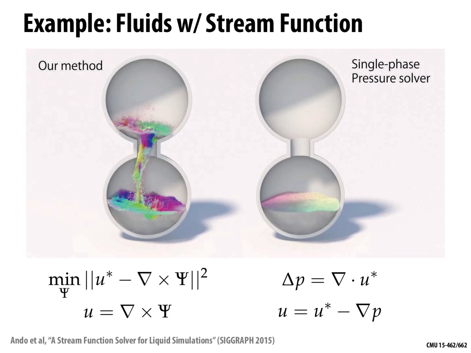
I also did not completely understand the problems with this method besides the point that the boundary between air and water has pressure p = 0 which "does not enforce incompressibility of the air phase," even for a two-phase solver, which makes sense since the single-phase solver in the slide looked like it only simulated the flow of water down rather than the flow of air up.
In the context they provided, their results that
• Our resulting flow is guaranteed to be divergence-free regardless
of the accuracy of the solve.
• Our approach enforces incompressibility even in the unsimulated
air phase, enabling realistic two-phase flow simulation
by computing only a single phase
seem almost like magic :0
keenan
@jzhanson Rather than try to answer all your questions directly, I'll just point you to Robert Bridson's course notes, which are a great intro to fluid simulation in computer graphics.
ljelenak
I find it interesting that even though both of these methods essentially "solve" the same thing, that one is way more accurate in solving the problem realistically. Are the other cases in that both solutions are "correct" but one leads to a better result? Or was it actually that the solution on the right was incorrect all along?
xTheBHox
It still truly baffles me how the system on the left could be simulated, given that it's such a chaotic system. Intuitively it seems like a very small change in initial conditions could give rise to radically different simulations, which would mean that slight approximations in variables due to limited precision ought to cause the system to change a lot, making the simulation unrealistic; and yet it looks realistic.
keenan
@ljelenak All solutions are inaccurate, but some algorithms give more accurate solutions than others. Or, some algorithms are better at approximating one quantity (say, vorticity) than another (say, total energy), and vice versa. The trick in simulation is figuring out which quantity is most important for the task at hand. For instance, in graphics you might wish to pick algorithms that accurately simulate visual phenomena, or acoustic phenomena, depending on what you're doing (video vs. sound synthesis). E.g., solvers based on modal vibrations may be appropriate for small displacements at high frequencies (needed for sound synthesis), but not as useful for large, highly localized deformations (which might be needed for visual synthesis).
keenan
@xTheBHox Whether the equations of fluid motion are formally chaotic is unclear to me, though certainly many of the PDEs in graphics have significant instabilities. The saving grace is that the real-life phenomena they model are also unstable. So, people are used to seeing systems whose behavior depends in a sensitive way on the initial conditions---hence, if your algorithm is also sensitive in this way, it still provides a visually compelling solution. In other words, human beings aren't particularly adept at mapping initial conditions to long-term solutions, since they can't solve unstable PDEs in their heads! ;-). This is one of many places where human perception and computation meet in graphics.
Pretty colors! I looked up and skimmed the paper, and it was almost completely incomprehensible to me, but what it seems like the big picture of how fluids are simulated are using physics laws (and some environmental attributes, like walls of containers and so on) as constraints in a linear system where we are trying to minimize the kinetic energy, or as they describe more intuitively in the Introduction: "...find a pressure p whose gradient projects the velocity field into a divergence-free state."
Does that mean that we are looking for some pressure vector that makes the fluid behave in a state of "equilibrium" where there are no major differences in the velocity of the fluid due to pressure differences?
I also did not completely understand the problems with this method besides the point that the boundary between air and water has pressure p = 0 which "does not enforce incompressibility of the air phase," even for a two-phase solver, which makes sense since the single-phase solver in the slide looked like it only simulated the flow of water down rather than the flow of air up.
In the context they provided, their results that
• Our resulting flow is guaranteed to be divergence-free regardless of the accuracy of the solve. • Our approach enforces incompressibility even in the unsimulated air phase, enabling realistic two-phase flow simulation by computing only a single phase
seem almost like magic :0
@jzhanson Rather than try to answer all your questions directly, I'll just point you to Robert Bridson's course notes, which are a great intro to fluid simulation in computer graphics.
I find it interesting that even though both of these methods essentially "solve" the same thing, that one is way more accurate in solving the problem realistically. Are the other cases in that both solutions are "correct" but one leads to a better result? Or was it actually that the solution on the right was incorrect all along?
It still truly baffles me how the system on the left could be simulated, given that it's such a chaotic system. Intuitively it seems like a very small change in initial conditions could give rise to radically different simulations, which would mean that slight approximations in variables due to limited precision ought to cause the system to change a lot, making the simulation unrealistic; and yet it looks realistic.
@ljelenak All solutions are inaccurate, but some algorithms give more accurate solutions than others. Or, some algorithms are better at approximating one quantity (say, vorticity) than another (say, total energy), and vice versa. The trick in simulation is figuring out which quantity is most important for the task at hand. For instance, in graphics you might wish to pick algorithms that accurately simulate visual phenomena, or acoustic phenomena, depending on what you're doing (video vs. sound synthesis). E.g., solvers based on modal vibrations may be appropriate for small displacements at high frequencies (needed for sound synthesis), but not as useful for large, highly localized deformations (which might be needed for visual synthesis).
@xTheBHox Whether the equations of fluid motion are formally chaotic is unclear to me, though certainly many of the PDEs in graphics have significant instabilities. The saving grace is that the real-life phenomena they model are also unstable. So, people are used to seeing systems whose behavior depends in a sensitive way on the initial conditions---hence, if your algorithm is also sensitive in this way, it still provides a visually compelling solution. In other words, human beings aren't particularly adept at mapping initial conditions to long-term solutions, since they can't solve unstable PDEs in their heads! ;-). This is one of many places where human perception and computation meet in graphics.