I understand dividing by p is necessary for averaging samples, but how can we prove the result is just “?" integration instead of the expression multiplies some scalar things? Mathematical proof seems to be not easy since p(X) is probability distribution instead of probability.
echo
The missing sign is "approximates"
lykospirit
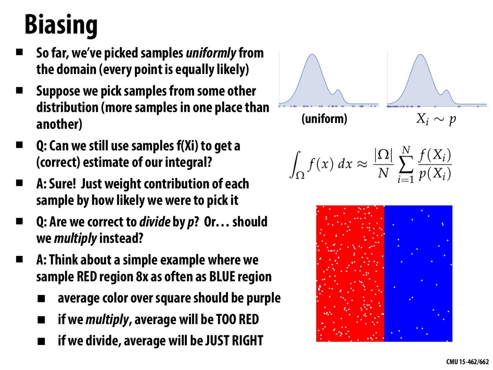
I was wondering about this too: the red/blue example makes sense with a discrete probability distribution, but how does this work with a continuous one?
Is the p(X_i) in the expression for the Monte Carlo integral a "discretized" version of the probability distribution? Like in the red/blue example, for any point (x,y) in [0,1]^2, we assign p(X_i)=8/9 if x<1/2, p(X_i)=1/9 if x>=1/2?
mdsavage
In the discrete case, what we're trying to compute is:
sum [x in omega] f(x)
So if we sample a point x with probability p(x), then we need to account for that by dividing by the sampling probability, and then taking n samples we get:
(|omega| / n) sum[i = 1..n] (f(x_i) / p(x_i))
The same logic should apply in the continuous case, so we're trying to compute:
integral [x in omega] f(x)
Again, we need to account for our sampling bias. The weight with which each point biases the sample is exactly its value in the probability density function, so we again divide by that. We then take the same approach to approximating as before, and end up with the same result.
So @lykospirit, assuming this intuition is correct, that should work so long as the area of the red and blue rectangles are each 1 (so the integral of p(x) over the entire area is 1, so it's a valid PDF).
I understand dividing by p is necessary for averaging samples, but how can we prove the result is just “?" integration instead of the expression multiplies some scalar things? Mathematical proof seems to be not easy since p(X) is probability distribution instead of probability.
The missing sign is "approximates"
I was wondering about this too: the red/blue example makes sense with a discrete probability distribution, but how does this work with a continuous one?
Is the p(X_i) in the expression for the Monte Carlo integral a "discretized" version of the probability distribution? Like in the red/blue example, for any point (x,y) in [0,1]^2, we assign p(X_i)=8/9 if x<1/2, p(X_i)=1/9 if x>=1/2?
In the discrete case, what we're trying to compute is:
sum [x in omega] f(x)
So if we sample a point x with probability p(x), then we need to account for that by dividing by the sampling probability, and then taking n samples we get:
(|omega| / n) sum[i = 1..n] (f(x_i) / p(x_i))
The same logic should apply in the continuous case, so we're trying to compute:
integral [x in omega] f(x)
Again, we need to account for our sampling bias. The weight with which each point biases the sample is exactly its value in the probability density function, so we again divide by that. We then take the same approach to approximating as before, and end up with the same result.
So @lykospirit, assuming this intuition is correct, that should work so long as the area of the red and blue rectangles are each 1 (so the integral of p(x) over the entire area is 1, so it's a valid PDF).