What are some of the promising approaches to demystifying nonconvex optimization? Of course since it's NP-hard we won't be able to get a perfect solution, but do we have some reasonable approximations that carry certain theoretical guarantees or which work well in practice?
keenan
@jzhanson Good question. There has been steady progress in the past 15-20 years (give or take) in understanding convex optimization, with one of the most important insights being that large classes of convex problems can be solved efficiently (initially via interior point methods). The general understanding of nonconvex problems is not nearly as mature, but people are definitely pushing in this direction. I have a friend who runs the Facebook page on nonconvex optimization which may have some interesting pointers. At a practical level, it's also worth knowing about highly specialized examples of nonconvex problems that can nonetheless be solved efficiently; a very common one being eigenvalue problems, which show up extremely often in graphics (and elsewhere), though IIRC this can in some way be understood from a convex point of view... There are also, if I recall, some interesting examples of easily solvable nonconvex problems in Boyd and Vandenberghe's book.
siliangl
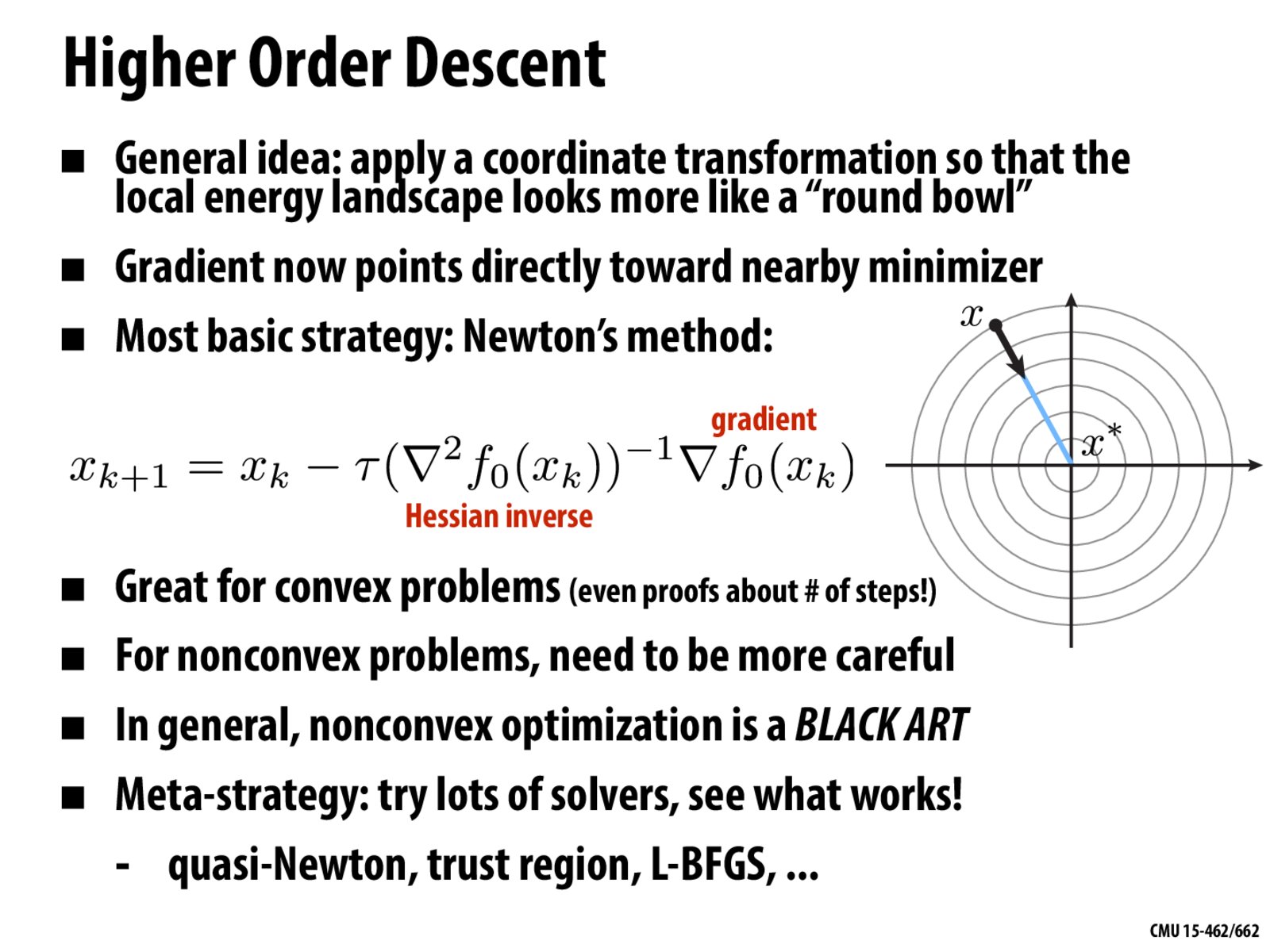
What kind of coordinate transformation would this be? Is it not the previous slide also having the energy landscape as a round bowl? What is the exact difference between the two?
mdsavage
@siliangl In this example, it looks like it was a composition of translation, rotation, and scaling, but I'd imagine other transformations would be valid as well.
The difference between this slide and the last one is that the gradients in this energy landscape all point roughly towards the local minimum, so we need fewer steps to converge (as opposed to the last slide, in which the gradients did not exhibit this property, so we had to spend many steps oscillating before converging).
keenan
@siliangl The coordinate transform is to apply the inverse of the Hessian to the gradient vector. (The Hessian is a matrix; its inverse represents a linear coordinate transformation.)
The reason this makes sense is that any nice enough function can be approximated by its Taylor series
So, if you apply the inverse of the Hessian the quadratic part will just look like a nice "round bowl" $(x-x_0)^T (x-x_0)$ plus some smaller junk. You no longer have to worry about finding your way down to the bottom of a "long skinny bowl" (as on the previous slide); just the junk.
What are some of the promising approaches to demystifying nonconvex optimization? Of course since it's NP-hard we won't be able to get a perfect solution, but do we have some reasonable approximations that carry certain theoretical guarantees or which work well in practice?
@jzhanson Good question. There has been steady progress in the past 15-20 years (give or take) in understanding convex optimization, with one of the most important insights being that large classes of convex problems can be solved efficiently (initially via interior point methods). The general understanding of nonconvex problems is not nearly as mature, but people are definitely pushing in this direction. I have a friend who runs the Facebook page on nonconvex optimization which may have some interesting pointers. At a practical level, it's also worth knowing about highly specialized examples of nonconvex problems that can nonetheless be solved efficiently; a very common one being eigenvalue problems, which show up extremely often in graphics (and elsewhere), though IIRC this can in some way be understood from a convex point of view... There are also, if I recall, some interesting examples of easily solvable nonconvex problems in Boyd and Vandenberghe's book.
What kind of coordinate transformation would this be? Is it not the previous slide also having the energy landscape as a round bowl? What is the exact difference between the two?
@siliangl In this example, it looks like it was a composition of translation, rotation, and scaling, but I'd imagine other transformations would be valid as well.
The difference between this slide and the last one is that the gradients in this energy landscape all point roughly towards the local minimum, so we need fewer steps to converge (as opposed to the last slide, in which the gradients did not exhibit this property, so we had to spend many steps oscillating before converging).
@siliangl The coordinate transform is to apply the inverse of the Hessian to the gradient vector. (The Hessian is a matrix; its inverse represents a linear coordinate transformation.)
The reason this makes sense is that any nice enough function can be approximated by its Taylor series
$ f(x) = f(x_0) + (x-x_0)^T \nabla f(x_0) + (x-x_0)^T \nabla^2 f(x_0) (x-x0) + O(|x-x_0|^3).$
So, if you apply the inverse of the Hessian the quadratic part will just look like a nice "round bowl" $(x-x_0)^T (x-x_0)$ plus some smaller junk. You no longer have to worry about finding your way down to the bottom of a "long skinny bowl" (as on the previous slide); just the junk.