Overview

This document describes the internal data structures and algorithms that comprise the Scotty3D codebase, focusing mainly on core functionality (e.g., meshing and ray tracing). Limited documentation of the graphical user interface (GUI) is available via comments in the source itself (though this information is not needed for assignments).

Geometric Data Structures

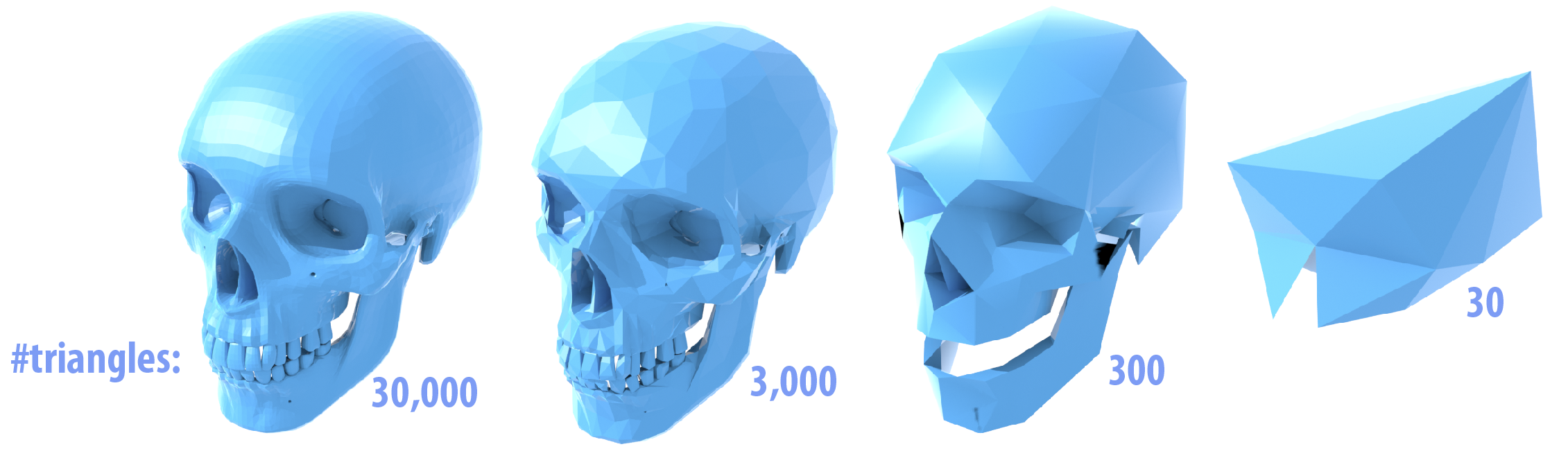
Scotty3D uses a variety of geometric data structures, depending on the task. Some operations (e.g., ray tracing) use a simple list of triangles that can be compactly encoded and efficiently cached. For more sophisticated geometric tasks like mesh editing and sampling, a simple triangle list is no longer sufficient (or leads to unnecessarily poor asymptotic performance). Most actions in MeshEdit mode therefore use a topological data structure called a halfedge mesh (also known as a _doubly-connected edge list), which provides a good tradeoff between simplicity and sophistication.

The Halfedge Data Structure

The basic idea behind the halfedge data structure is that, in addition to the usual vertices, edges, and faces that make up a polygonal mesh, we also have an entity called a halfedge that acts like "glue" connecting the different elements. It is this glue that allow us to easily "navigate" the mesh, i.e., easily access mesh elements adjacent to a given element.

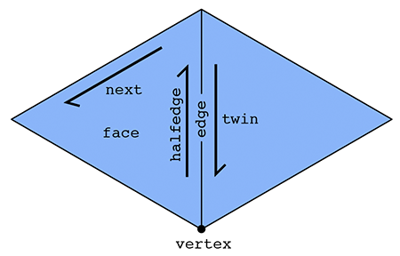
In particular, there are two halfedges associated with each edge (see picture above). For an edge connecting two vertices i and j, one of its halfedges points from i to j; the other one points from j to i. In other words, we say that the two halfedges are oppositely oriented. On of the halfedges is associated with the face to the "left" of the edge; the other is associated with the face to the "right." Each halfedge knows about the opposite halfedge, which we call its twin. It also knows about the next halfedge around its face, as well as its associated edge, face, and vertex.

In contrast, the standard mesh elements (vertices, edges, and faces) know only about one of their halfedges. In particular:

• a vertex knows about one of its "outgoing" halfedges,
• an edge knows about one of its two halfedges, and
• a face knows about one of the many halfedges circulating around its interior.

In summary, we have the following relationships:

Mesh element	Pointers
Vertex	one halfedge
Edge	one halfedge
Face	one halfedge
Halfedge	twin, next, vertex, edge, face

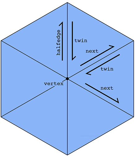
This list emphasizes that it is really the halfedges that connect everything up. An easy example is if we want to visit all the vertices of a given face. We can start at the face's halfedge, and follow the "next" pointer until we're back at the beginning. A more interesting example is visiting all the vertices adjacent to a given vertex v. We can start by getting its outgoing halfedge, then its twin, then its next halfedge; this final halfedge will also point out of vertex v, but it will point toward a different vertex than the first halfedge. By repeating this process, we can visit all the neighboring vertices:

In some sense, a halfedge mesh is kind of like a linked list on steroids. For instance, the halfedges around a given face (connected by next pointers) form a sort of "cyclic" linked list, where the tail points back to the head.

A nice consequence of the halfedge representation is that any valid halfedge mesh must be manifold and orientable. Scotty3D will therefore only produce manifold, oriented meshes as output (and will complain if the input does not satisfy these criteria).

The HalfedgeMesh Class

The Scotty3D skeleton code already provides a fairly sophisticated implementation of the half edge data structure, in the HalfedgeMesh class (see halfEdgeMesh.h and halfEdgeMesh.cpp). Although the detailed implementation may appear a bit complicated, the basic interface is not much different from the abstract description given above. For instance, suppose we have a face f and want to print out the positions of all its vertices. We would write a routine like this:

void printVertexPositions(FaceCIter f) {
  HalfEdgeCIter h = f->halfedge(); // get the first halfedge of the face
  do {
    VertexCIter v = h->vertex();   // get the vertex of the current halfedge
    cout << v->position << endl;   // print the vertex position
    h = h->next();                 // move to the next halfedge around the face
  } while (h != f->halfedge());    // keep going until we're back at the beginning
}

Notice that we refer to a face as a FaceCIter rather than just a Face. You can think of an Iter as a kind of pointer; the letter C indicates that this pointer is "constant", i.e., for this particular algorithm, we will not change the value pointed to by f. Note that members of an iterator are accessed with an arrow -> rather than a dot ., just as with pointers. (A more in-depth explanation of some of these details can be found in the inline documentation.) Similarly, to print out the positions of all the neighbors of a given vertex we could write a routine like this:

void printNeighborPositions(VertexCIter v) {
  HalfEdgeCIter h = v->halfedge();    // get one of the outgoing halfedges of the vertex
  do {
    HalfEdgeCIter h_twin = h->twin(); // get the vertex of the current halfedge
    VertexCIter v = h_twin->vertex(); // vertex is 'source' of the half edge.
                                      // so h->vertex() is v,
                                      // whereas h_twin->vertex() is the neighbor vertex.
    cout << v->position << endl;      // print the vertex position
    h = h_twin->next();               // move to the next outgoing halfedge of the vertex.
  } while(h != v->halfedge());        // keep going until we're back at the beginning
}

To iterate over all the vertices in a halfedge mesh, we could write a loop like this:

for(VertexCIter v = mesh.verticesBegin(); v != mesh.verticesEnd(); v++) {
  printNeighborPositions(v); // do something interesting here
}

Internally, the lists of vertices, edges, faces, and halfedges are stored as linked lists, which allows us to easily add or delete elements to our mesh. For instance, to add a new vertex we can write

VertexIter v = mesh.newVertex();

Likewise, to delete a vertex we can write

mesh.deleteVertex(v);

Note, however, that one should be very, very careful when adding or deleting mesh elements. New mesh elements must be properly linked to the mesh -- for instance, this new vertex must be pointed to one of its associated halfedges by writing something like

v->halfedge() = h;

Likewise, if we delete a mesh element, we must be certain that no existing elements still point to it; the halfedge data structure does not take care of these relationships for you automatically. In fact, that is exactly the point of this assignment: to get some practice directly manipulating the halfedge data structure. Being able to perform these low-level manipulations will enable you to write useful and interesting mesh code far beyond the basic operations in this assignment.

Finally, the boundary of the surface (e.g., the ankles and waist of a pair of pants) requires special care in our halfedge implementation. At first glance, it would seem that the routine printNeighborPositions() above might break if the vertex v is on the boundary, because at some point we worry that we have no twin() element to visit. Fortunately, our implementation has been designed to avoid this kind of catastrophe. In particular, rather than having an actual hole in the mesh, we create a "virtual" boundary face whose edges are all the edges of the boundary loop. This way, we can iterate over boundary elements just like any other mesh element. If we ever need to check whether an element is on the boundary, we have the methods.

Vertex::isBoundary()
Edge::isBoundary()
Face::isBoundary()
Halfedge::isBoundary()

These methods return true if and only if the element is contained in the domain boundary. Additionally, we store an explicit list of boundary faces, which we can iterate over like any other type of mesh element:

for(FaceCIter b = mesh.boundariesBegin(); b != mesh.boundariesEnd(); b++) {
  // do something interesting with this boundary loop
}

These virtual faces are not stored in the usual face list, i.e., they will not show up when iterating over faces. The figure below should help to further explain the behavior of HalfedgeMesh for surfaces with boundary:

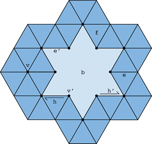
Dark blue regions indicate interior faces, whereas light blue regions indicate virtual boundary faces. A vertex, edge, or halfedge is considered to be part of the boundary if it is contained entirely in a boundary face. For instance, in the figure above the region b is a virtual boundary face, which means that vertex v', edge e', and halfedge h' are all part of the boundary; their isBoundary() methods will return true. In contrast, vertex v, edge e, face f, and halfedge h are not part of the boundary, and their isBoundary() methods will return false. Notice also that the boundary face b is a polygon with 12 edges.

Note: the edge degree and face degree of a boundary vertex is not the same! Notice, for instance, that vertex v' is contained in three edges but only two interior faces. By convention, Vertex::degree() returns the face degree, not the edge degree. The edge degree can be computed by finding the face degree, and adding 1 if the vertex is a boundary vertex.

Please refer to the inline comments for further details about the HalfedgeMesh data structure.

Tutorial: Local Mesh Operations

Many of the actions that need to be implemented in the MeshEdit mode are local mesh operations (like edge collapse, face bevel, etc.). Here we provide a step-by-step guide to implementing a simplied version of the EdgeFlip operation for a pair of triangles---the final version, however, must be implemented for general polygons (i.e., any $n$-gon). The basic strategy for implementing the other local operations is quite similar to the procedure outlined below. Note: if you're not familiar with C++, you should definitely take a moment to learn about the standard library class std::vector, especially the method push_back(), which will make it easy to accumulate a list of pointers as you walk around a polygon, vertex, etc.

A good recipe for ensuring that all pointers are still valid after a local remeshing operation is:

1. Draw a picture of all the elements (vertices, edges, faces, halfedges) that will be needed from the original mesh, and all the elements that should appear in the modified mesh.
2. Allocate any new elements that are needed in the modified mesh, but do not appear in the original mesh.
3. For every element in the "modified" picture, set all of its pointers -- even if they didn't change. For instance, for each halfedge, make sure to set next, twin, vertex, edge, and face to the correct values in the new (modified) picture. For each vertex, make sure to set its halfedge pointer. Etc. A convenience method Halfedge::setNeighbors() has been created for this purpose.
4. Deallocate any elements that are no longer used in the modified mesh, which can be done by calling HalfedgeMesh::deleteVertex(), HalfedgeMesh::deleteEdge(), etc.

The reason for setting all the pointers (and not just the ones that changed) is that it is very easy to miss a pointer, causing your code to crash. Once the code is working, you can remove these unnecessary assignments if you wish -- but remember that premature optimization is the root of all evil

We now consider the case of a triangle-triangle edge flip.

PHASE 0: Draw a Diagram

Suppose we have a pair of triangles (a,b,c) and (c,b,d). After flipping the edge (b,c), we should now have triangles (a,d,c) and (a,b,d). A good first step for implementing any local mesh operation is to draw a diagram that clearly labels all elements affected by the operation:

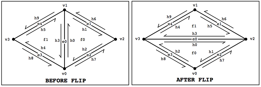
Here we have drawn a diagram of the region around the edge both before and after the edge operation (in this case, "flip"), labeling each type of element (halfedge, vertex, edge, and face) from zero to the number of elements. It is important to include every element affected by the operation, thinking very carefully about which elements will be affected. If elements are omitted during this phase, everything will break---even if the code written in the two phases is correct! In this example, for instance, we need to remember to include the halfedges "outside" the neighborhood, since their "twin" pointers will be affected.

PHASE I: Collect elements

Once you've drawn your diagram, simply collect all the elements from the "before" picture. Give them the same names as in your diagram, so that you can debug your code by comparing with the picture.

// HALFEDGES
HalfedgeIter h0 = e0->halfedge();
HalfedgeIter h1 = h0->next();
HalfedgeIter h2 = h1->next();
HalfedgeIter h3 = h0->twin();
HalfedgeIter h4 = h3->next();
HalfedgeIter h5 = h4->next();
HalfedgeIter h6 = h1->twin();
HalfedgeIter h7 = h2->twin();
HalfedgeIter h8 = h4->twin();
HalfedgeIter h9 = h5->twin();

// VERTICES
VertexIter v0 = h0->vertex();
VertexIter v1 = h3->vertex();
// ...you fill in the rest!...

// EDGES
e1 = h1->edge();
e2 = h2->edge();
// ...you fill in the rest!...

// FACES
f0 = h0->face();
// ...you fill in the rest!...

PHASE II: Allocate new elements

If your edge operation requires new elements, now is the time to allocate them. For the edge flip, we don't need any new elements; but suppose that for some reason we needed a new vertex v4. At this point we would allocate the new vertex via

VertexIter v4 = mesh.newVertex();

(The name used for this new vertex should correspond to the label you give it in your "after" picture.) Likewise, new edges, halfedges, and faces can be allocated via the methods mesh.newEdge(), mesh.newHalfedge(), and mesh.newFace().

PHASE III: Reassign Elements

Next, update the pointers for all the mesh elements that are affected by the edge operation. Be exhaustive! In other words, go ahead and specify every pointer for every element, even if it did not change. Once things are working correctly, you can always optimize by removing unnecessary assignments. But get it working correctly first! Correctness is more important than efficiency.

// HALFEDGES
h0->next() = h1;
h0->twin() = h3;
h0->vertex() = v3;
h0->edge() = e0;
h0->face() = f0;
h1->next() = h2;
h1->twin() = h7;
h1->vertex() = v2;
h1->edge() = e2;
h1->face() = f0;
// ...you fill in the rest!...

// ...and don't forget about the "outside" elements!...
h9->next() = h9->next(); // didn't change, but set it anyway!
h9->twin() = h4;
h9->vertex() = v1;
h9->edge() = e4;
h9->face() = h9->face(); // didn't change, but set it anyway!

// VERTICES
v0->halfedge() = h2;
v1->halfedge() = h5;
v2->halfedge() = h3;
v3->halfedge() = h0;

// EDGES
e0->halfedge() = h0; //...you fill in the rest!...

// FACES
f0->halfedge() = h0; //...you fill in the rest!...

PHASE IV: Delete unused elements

If your edge operation eliminates elements, now is the best time to deallocate them: at this point, you can be sure that they are no longer needed. For instance, since we do not need the vertex allocated in PHASE II, we could write

mesh.deleteVertex( v4 );

You should be careful that this mesh element is not referenced by any other element in the mesh. But if your "before" and "after" diagrams are correct, that should not be an issue!

Design considerations

The basic algorithm outlined above will handle most edge flips, but you should also think carefully about possible corner-cases. You should also think about other design issues, like "how much should this operation cost?" For instance, for this simple triangle-triangle edge flip it might be reasonable to:

• Ignore requests to flip boundary edges (i.e., just return immediately if either neighboring face is a boundary loop).
• Ignore requests to perform any edge flip that would make the surface non-manifold or otherwise invalidate the mesh.
• Not add or delete any elements. Since there are the same number of mesh elements before and after the flip, you should only need to reassign pointers.
• Perform only a constant amount of work -- the cost of flipping a single edge should not be proportional to the size of the mesh!

Formally proving that your code is correct in all cases is challenging, but at least try to think about what could go wrong in degenerate cases (e.g., vertices of low degree, or very small meshes like a tetrahedron). The biggest challenge in properly implementing this type of local operation is making sure that all the pointers still point to the right place in the modified mesh, and will likely be the cause of most of your crashes!

Beveling

Here we provide some additional detail about the bevel operations and their implementation in Scotty3D. Each bevel operation has two components:

1. a method that modifies the connectivity of the mesh, creating new beveled elements, and
2. a method the updates the geometry of the mesh, insetting and offseting the new vertices according to user input.

The methods that update the connectivity are HalfedgeMesh::bevelVertex, halfedgeMesh::bevelEdge, and HalfedgeMesh::bevelFace. The methods that update geometry are HalfedgeMesh::_bevel_vtx_reposition_with_dist, HalfedgeMesh::_bevel_edge_reposition_with_dist, and HalfedgeMesh::_bevel_fc_reposition_with_dist. The methods for updating connectivity can be implemented following the general strategy outlined in the tutorial above.

To update the geometry of a beveled element, you are provided with the following data:

• orig - These are the original vertex positions of the mesh element, before any insetting or offseting is applied.
• hs - These are the halfedges "around" the element currently being beveled.
• inset - The amount by which the new face should be inset (i.e., "shrunk" or "expanded")
• shift (faces only) - The amount by which the new face should be offset in the normal direction.

More specifically, the array hs stores the following data:

• For a beveled vertex, hs stores the halfedges pointing from the vertices of the new polygon to the neighbors of the original vertex.
• For a beveled edge, hs stores the halfedges pointing from the vertices of the new polygon to the neighbors of the original edge endpoints.
• For a beveled face, hs stores the halfedges pointing from the vertices of the new polygon to the vertices of the original polygon.

These relationships are illustrated by the following diagram:

The basic recipe for updating the vertex positions is then:

• Iterate over the list of halfedges (hs)
• Grab the vertex coordinates that are needed to compute the new, updated vertex coordinates (this could be a mix of values from orig, or the members Vertex::position)
• Compute the updated vertex positions using the current values of inset (and possibly shift)
• Store the new vertex positions in Vertex::position for the vertices of the new, beveled polygon only (i.e., the positions of any polygon "outside" the dark blue one in the figures above should not be updated)

The reason for storing hs and orig in an array is that it makes it easy to access positions "to the left" and "to the right" of a given vertex. For instance, suppose we want to figure out the offset from the corner of a polygon. We might want to compute some geometric quantity involving the three vertex positions orig[i-1], orig[i], and orig[i+1] (as well as inset), then set the new vertex position hs[i]->vertex()->position to this new value:

A useful trick here is modular arithmetic: since we really have a "loop" of vertices, we want to make sure that indexing the next element (+1) and the previous element (-1) properly "wraps around." This can be achieved via code like

// Get the number of vertices in the new polygon
int N = hs.size();

// Assuming we're looking at vertex i, compute the indices
// of the next and previous elements in the list using
// modular arithmetic---note that to get the previous index,
// we can't just subtract 1 because the mod operation in C++
// doesn't behave quite how you might expect for negative
// values!
int a = (i+N-1) % N;
int b = i;
int c = (i+1) % N;

// Get the actual 3D vertex coordinates at these vertices
Vector3D pa = orig[a];
Vector3D pb = orig[b];
Vector3D pc = orig[c];

From here, you will need to compute new coordinates for vertex i, which can be accessed from hes[i]->vertex()->position. As a "dummy" example (i.e., this is NOT what you should actually do!!) this code will set the position of the new vertex to the average of the vertices above:

hes[i].vertex()->position = ( pa + pb + pc ) / 3.; // replace with something that actually makes sense!

The only question remaining is: where should you put the beveled vertex? We will leave this decision up to you. This question is one where you will have to think a little bit about what a good design would be. Questions to ask yourself:

• How do I compute a point that is inset from the original geometry?
• For faces, how do I shift the geometry in the normal direction? (You may wish to use the method Face::normal() here.)
• What should I do as the offset geometry starts to look degenerate, e.g., shrinks to a point, or goes outside some reasonable bounds?
• What should I do when the geometry is nonplanar?
• Etc.

The best way to get a feel for whether you have a good design is to try it out! Can you successfully and easily use this tool to edit your mesh? Or is it a total pain, producing bizarre results? You be the judge!

Interface with global mesh operations

To facilitate user interaction, as well as global mesh processing operations (described below), local mesh operations should return the following values when possible. If the specified values are not available, you should think about a reasonable alternative value to return. First and foremost, the program should not crash! So for instance, you should not return a pointer to an element that was deleted. Second, you should try as much as possible to return a value related to the argument. For instance, if the user asks to flip an edge e that cannot be flipped (e.g., a boundary edge), the most natural solution would be to simply return e. Likewise, if the user asks to erase an edge e that cannot be erased, a natural return value might be an adjacent (non-boundary) face. Etc.

• HalfedgeMesh::flipEdge - should return the edge that was flipped
• HalfedgeMesh::splitEdge - should return the inserted vertex
• HalfedgeMesh::collapseEdge - should return the new vertex, corresponding to the collapsed edge
• HalfedgeMesh::collapseFace - should return the new vertex, corresponding to the collapsed face
• HalfedgeMesh::eraseVertex - should return the new face, corresponding to the faces originally containing the vertex
• HalfedgeMesh::eraseEdge - should return the new face, corresponding to the faces originally containing the edge
• HalfedgeMesh::bevelVertex - should return the new face, corresponding to the beveled vertex
• HalfedgeMesh::bevelEdge - should return the new face, corresponding to the beveled edge
• HalfedgeMesh::bevelFace - should return the new, inset face

---

Global Mesh Processing

In addition to local operations on mesh connectivity, Scotty3D provides several global remeshing operations (as outlined in the User Guide). Two different mechanisms are used to implement global operations:

• Repeated application of local operations. Some mesh operations are most easily expressed by applying local operations (edge flips, etc.) to a sequence of mesh elements until the target output is achieved. A good example is mesh simplification, which is a greedy algorithm that collapses one edge at a time (see further discussion below).
• Global replacement of the mesh. Other mesh operations are better expressed by temporarily storing new mesh elements in a simpler mesh data structure (e.g., an indexed list of faces) and completely re-building the halfedge data structure from this data. A good example is Catmull-Clark subdivision, where every polygon must be simultaneously split into quadrilaterals (see further discussion below).

Note that in general there are no inter-dependencies among global remeshing operations (except that some of them require a triangle mesh as input, which can be achieved via the method HalfedgeMesh::triangulate).

As a sanity check, each of your resampling algorithms should complete almost instantaneously (no more than a second or so) on meshes of a few hundred polygons. If performance is significantly worse than this, you may be repeatedly iterating over more elements than you really need to, or allocating/deallocating more memory than necessary. A useful debugging technique is to print out (or otherwise keep track of, e.g., via an integer counter or a profiler) the number of times basic methods like Halfedge::next() or HalfedgeMesh::newVertex() are called during a single execution of one of your methods; for most methods this number should be some reasonably small constant (no more than, say, 1000!) times the number of elements in the mesh.

---

Triangulation

A variety of geometry processing algorithms become easier to implement (or are only well defined) when the input consists purely of triangles. The method HalfedgeMesh::triangulate converts any polygon mesh into a triangle mesh by splitting each polygon into triangles. This transformation is performed in-place, i.e., the original mesh data is replaced with the new, triangulated data (rather than making a copy). The triangulate method is basically just a wrapper around HalfedgeMesh::splitPolygon, which splits a single face f into triangles. The implementation of this method will look much like the implementation of the local mesh operations (see the tutorial above).

There is more than one way to split a polygon into triangles. Two common patterns are to connect every vertex to a single vertex, or to "zig-zag" the triangulation across the polygon:

The splitPolygon routine is not required to produce any particular triangulation so long as:

• all polygons in the output are triangles,
• the vertex positions remain unchanged, and
• the output is a valid, manifold halfedge mesh.

Note that triangulation of nonconvex or nonplanar polygons may lead to geometry that is unattractive or difficult to interpret. However, the purpose of this method is simply to produce triangular connectivity for a given polygon mesh, and correct halfedge connectivity is the only invariant that must be preserved by the implementation. The geometric quality of the triangulation can later be improved by running other global algorithms (e.g., isotropic remeshing); ambitious developers may also wish to consult the following reference:

• Zou et al, "An Algorithm for Triangulating Multiple 3D Polygons"

---

Subdivision

In image processing, we often have a low resolution image that we want to display at a higher resolution. Since we only have a few samples of the original signal, we need to somehow interpolate or upsample the image. One idea would be to simply cut each pixel into four, leaving the color values unchanged, but this leads to a blocky appearance. Instead we might try a more sophisticated scheme (like bilinear or trilinear interpolation) that yields a smoother appearance.

In geometry processing, one encounters the same situation: we may have a low-resolution polygon mesh that we wish to upsample for display, simulation, etc. Simply splitting each polygon into smaller pieces doesn't help, because it does nothing to alleviate blocky silhouettes or chunky features. Instead, we need an upsampling scheme that nicely interpolates or approximates the original data. Polygon meshes are quite a bit trickier than images, however, since our sample points are generally at irregular locations, i.e., they are no longer found at regular intervals on a grid.

Three subdivision schemes are supported by Scotty3D: Linear, Catmull-Clark, and Loop. The first two can be used on any polygon mesh, and should be implemented via the global replacement strategy described above. Loop subdivision can be implemented using repeated application of local oeprations. See further details below.

Linear subdivision

Although our ultimate goal is to produce a smooth approximation of the control cage, the first step is to simply update the connectivity (but not the vertex positions) so that the mesh has a larger number of elements. This kind of basic splitting or "linear subdivision" is also useful for box modeling, when we simply want to increase the number of available control points.

Unlike most of the other global remeshing operations, linear (and Catmull-Clark) subdivision will proceed by completely replacing the original halfedge mesh with a new one. The high-level procedure is:

1. Generate a list of vertex positions for the new mesh.
2. Generate a list of polygons for the new mesh, as a list of indices into the new vertex list (a la "polygon soup").
3. Hand these two lists to the method HalfedgeMesh::rebuild, which rebuilds the halfedge connectivity from scratch.

Given these lists, rebuild will take care of allocating halfedges, setting up next and twin pointers, etc., based on the list of polygons generated in step 2---this routine is already implemented in the Scotty3D skeleton code.

Both linear and Catmull-Clark subdivision schemes will handle general $n$-gons (i.e., polygons with $n$ sides) rather than, say, quads only or triangles only. Each $n$-gon (including but not limited to quadrilaterals) will be split into $n$ quadrailaterals according to the following template:

The high-level procedure is outlined in greater detail in HalfedgeMesh::subdivideQuad.

Vertex positions

For global linear or Catmull-Clark subdivision, the strategy for assigning new vertex positions may at first appear a bit strange: in addition to updating positions at vertices, we will also calculate vertex positions associated with the edges and faces of the original mesh. Storing new vertex positions on edges and faces will make it extremely convenient to generate the polygons in our new mesh, since we can still use the halfedge data structure to decide which four positions get connected up to form a quadrilateral. In particular, each quad in the new mesh will consist of:

• one new vertex associated with a face from the original mesh,
• two new vertices associated with edges from the original mesh, and
• one vertex from the original mesh.

For linear subdivision, the rules for computing new vertex positions are very simple:

• New vertices at original faces are assigned the average coordinates of all corners of that face (i.e., the arithmetic mean).
• New vertices at original edges are assigned the average coordinates of the two edge endpoints.
• New vertices at original vertices are assigned the same coordinates as in the original mesh.

These values should be assigned to the members Face::newPosition, Edge::newPosition, and Vertex::newPosition, respectively. For instance, f->newPosition = Vector3D( x, y, z ); will assign the coordinates (x,y,z) to the new vertex associated with face f. The general strategy for assigning these new positions is to iterate over all vertices, then all edges, then all faces, assigning appropriate values to newPosition. Note: you must copy the original vertex position Vertex::position to the new vertex position Vertex::newPosition; these values will not be used automatically.

This step should be implemented in the method HalfedgeMesh::computeLinearSubdivisionPositions in meshEdit.cpp.

Once the new vertex positions have been assigned to elements of the halfedge mesh, they need to be accumulated into a single list of all vertex positions in the new mesh, which will be handed to HalfedgeMesh::rebuild. It is important that vertex coordinates in this list appear in the same order they were indexed! For instance, if you index vertices, then edges, then faces, then the final vertex coordinate list should likewise contain coordinates from vertices, then coordinates from edges, then coordinates from faces. These vertex coordinates can be accumuluated using an object of type vector<Vector3D>, i.e., a dynamically-sized array of vertex positions. The basic strategy is to loop over all vertices, then all edges, then all faces, calling push_back to append each new vertex coordinate to the list. (See the next section for further discussion of the vector class.) Further details are provided in the in-line comments.

This last step should be implemented in the method HalfedgeMesh::buildSubdivisionVertexList in meshEdit.cpp.

Vertex indices

In addition to new (x,y,z) coordinates, we also need to assign a unique index to each vertex in the new mesh---including those that are associated with edges and faces. In other words, every vertex, edge, and face in the mesh will be assigned an integer between 0 and $N-1$, where $N$ is the total number of vertices plus edges plus faces in the original mesh. A simple strategy for assigning these indices is:

1. Initialize a counter to zero.
2. Iterate over vertices, assigning the index of the current vertex to the counter value, and incrementing the counter.
3. Iterate over edges, assigning the index of the current edge to the counter value, and incrementing the counter.
4. Iterate over faces, assigning the index of the current face to the counter value, and incrementing the counter.

Note that the particular choice of indices does not matter---the only things you must guarantee are that (i) every mesh element is assigned a valid index, and (ii) no two mesh elements share the same index.

Polygons

Unlike the local operations described above, which are applied one element after another, in linear and Catmull-Clark subdivision all polygons are subdivided simultaneously. In other words, if we focus on the whole mesh (rather than a single polygon), then we are

• creating one new vertex for each edge,
• creating one new vertex for each face, and
• keeping all the vertices of the original mesh.

These vertices are then connected up to form quadrilaterals ($n$ quadrilaterals for each $n$-gon). Rather than directly modifying the halfedge connectivity, new quads will be collected in a much simpler mesh data structure: a list of polygons. Note that with this subdivision scheme, every polygon in the output mesh will be a quadrilateral, even if the input contains triangles, pentagons, etc.

In Scotty3D, a list of polygons can be declared as

vector< vector<Index> > quads;

where vector is a class from the C++ standard template library, representing a dynamically-sized array. An Index is just another name for a size_t, which is the standard C++ type for integers that specify an element of an array. Polygons can be created by allocating a list of appropriate size, then specifying the indices of each vertex in the polygon. For example:

vector<Index> quad( 4 ); // allocate an array with four elements
// Build a quad with vertices specified by integers (a,b,c,d), starting at zero.
// These indices should correspond to the indices computing when assigning vertex
// positions, as described above.
quad[0] = a;
quad[1] = b;
quad[2] = c;
quad[3] = d;

Once a quad has been created, it can be added to the list of quads by using the method vector::push_back, which appends an item to a vector:

vector< vector<Index> > newPolygons;
newPolygons.push_back( quad );

The full array of new polygons will then be passed to the method HalfedgeMesh::rebuild, together with the new vertex positions.

This step should be implemented in the method HalfedgeMesh::buildSubdivisionFaceList in meshEdit.cpp.

Catmull-Clark subdivision

The only difference between Catmull-Clark and linear subdivision is the choice of positions for new vertices. Whereas linear subdivision simply takes a uniform average of the old vertex positions, Catmull-Clark uses a very carefully-designed weighted average to ensure that the surface converges to a nice, round surface as the number of subdivision steps increases. The original scheme is described in the paper ``Recursively generated B-spline surfaces on arbitrary topological meshes'' by (Pixar co-founder) Ed Catmull and James Clark. Since then, the scheme has been thoroughly discussed, extended, and analyzed; more modern descriptions of the algorithm may be easier to read, including those from the Wikipedia and this webpage. In short, the new vertex positions can be calculated by:

1. setting the new vertex position at each face f to the average of all its original vertices (exactly as in linear subdivision),
2. setting the new vertex position at each edge e to the average of the new face positions (from step 1) and the original endpoint positions, and
3. setting the new vertex position at each vertex v to the weighted sum

$$ \frac{Q + 2R + (n-3)S}{n}, $$

where $n$ is the degree of vertex $v$ (i.e., the number of faces containing $v$), and

• $Q$ is the average of all new face position for faces containing $v$,
• $R$ is the average of all new edge positions for edges containing $v$, and
• $S$ is the original vertex position for vertex $v$.

In other words, the new vertex positions are an "average of averages." (Note that you will need to divide by $n$ both when computing $Q$ and $R$, and when computing the final, weighted value---this is not a typo!)

Apart from changing the way vertex positions are computed, there should be no difference in your implementation of linear and Catmull-Clark subdivision.

This step should be implemented in the method HalfedgeMesh::computeCatmullClarkPositions in meshEdit.cpp.

Loop subdivision

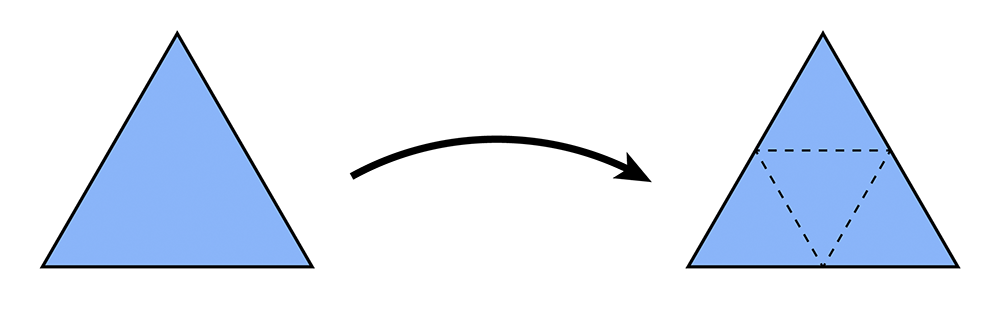
Loop subdivision (named after Charles Loop) is a standard approximating subdivision scheme for triangle meshes. At a high level, it consists of two basic steps:

1. Split each triangle into four by connecting edge midpoints (sometimes called "4-1 subdivision").
2. Update vertex positions as a particular weighted average of neighboring positions.

The 4-1 subdivision looks like this:

And the following picture illustrates the weighted average:

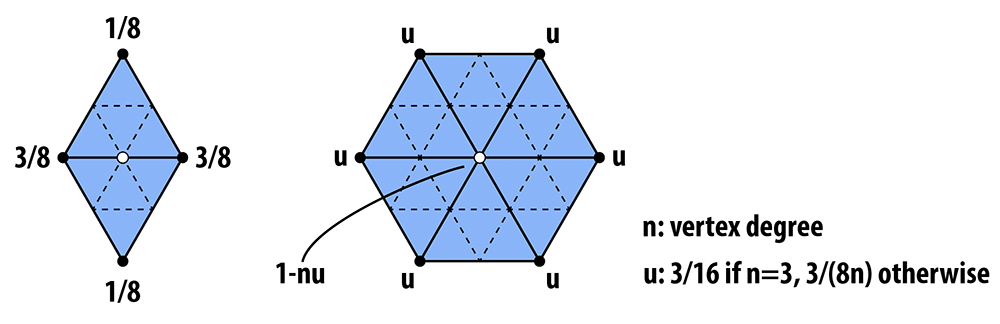
In words, the new position of an old vertice is (1 - nu) times the old position + u times the sum of the positions of all of its neighbors. The new position for a newly created vertex v that splits Edge AB and is flanked by opposite vertices C and D across the two faces connected to AB in the original mesh will be 3/8 * (A + B) + 1/8 * (C + D). If we repeatedly apply these two steps, we will converge to a fairly smooth approximation of our original mesh.

In contrast to linear and Catmull-Clark subdivision, Loop subdivision should be implemented using the local mesh operations described above (simply because it provides an alternative perspective on subdivision implementation, which can be useful in different scenarios). In particular, 4-1 subdivision can be achieved by applying the following strategy:

1. Split every edge of the mesh in any order whatsoever.
2. Flip any new edge that touches a new vertex and an old vertex.

The following pictures (courtesy Denis Zorin) illustrate this idea:

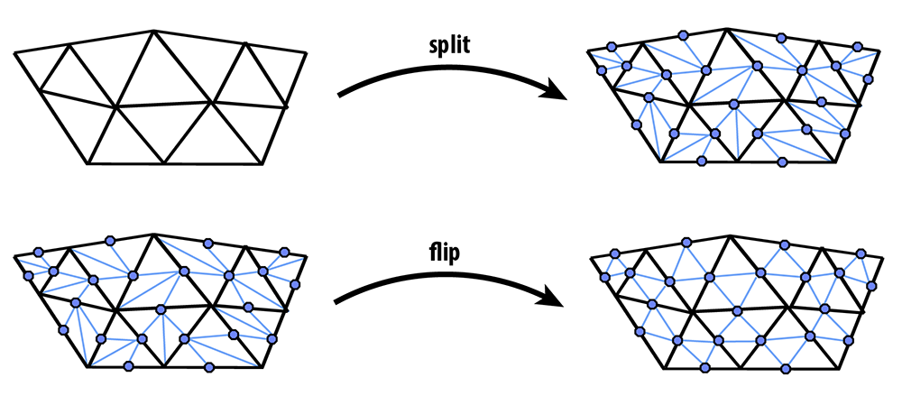
Notice that only blue (and not black) edges are flipped in this procedure; as described above, edges in the split mesh should be flipped if and only if they touch both an original vertex and a new vertex (i.e., a midpoint of an original edge).

When working with dynamic mesh data structures (like a halfedge mesh), one must think very carefully about the order in which mesh elements are processed---it is quite easy to delete an element at one point in the code, then try to access it later (typically resulting in a crash!). For instance, suppose we write a loop like this:

// iterate over all edges in the mesh
for (EdgeIter e = mesh.edgesBegin(); e != mesh.edgesEnd(); e++) {
  if (some condition is met) {
    mesh.splitEdge(e);
  }
}

Although this routine looks straightforward, it can very easily crash! The reason is fairly subtle: we are iterating over edges in the mesh by incrementing the iterator e (via the expression e++). But since splitEdge() is allowed to create and delete mesh elements, it might deallocate the edge pointed to by e before we increment it! To be safe, one should instead write a loop like this:

// iterate over all edges in the mesh
int n = mesh.nEdges();
EdgeIter e = mesh.edgesBegin();
for (int i = 0; i < n; i++) {

  // get the next edge NOW!
  EdgeIter nextEdge = e;
  nextEdge++;

  // now, even if splitting the edge deletes it...
  if (some condition is met) {
    mesh.splitEdge(e);
  }

  // ...we still have a valid reference to the next edge.
  e = nextEdge;
}

Note that this loop is just one example -- in general, you should think about which elements might be affected by a local mesh operation when writing your loops. Likewise, you can make life easier on yourself by making sure that your atomic edge operations provide certain guarantees. For instance, if your implementation of HalfedgeMesh::flipEdge() guarantees that no edges will be created or destroyed (as it should), then you can safely do edge flips inside a loop without worrying about these kinds of side effects.

For Loop subdivision, there are some additional data members that will make it easy to keep track of the data needed to update the connectivity and vertex positions. In particular:

• Vertex::newPosition can be used as temporary storage for the new position (computed via the weighted average above). Note that you should not change the value of Vertex::position until all the new vertex positions have been computed -- otherwise, you are taking averages of values that have already been averaged!
• Likewise, Edge::newPosition can be used to store the position of the vertices that will ultimately be inserted at edge midpoints. Again, these values should be computed from the original values (before subdivision), and applied to the new vertices only at the very end. The Edge::newPositionvalue will be used for the position of the vertex that will appear along the old edge after the edge is split. We precompute the position of the new vertex before splitting the edges and allocating the new vertices because it is easier to tansverse the simpler original mesh to find the positions for the weighted average that determines the positions of the new vertices.
• Vertex::isNew can be used to flag whether a vertex was part of the original mesh, or is a vertex newly inserted by subdivision (at an edge midpoint).
• Edge::isNew likewise flags whether an edge is a piece of an edge in the original mesh, or is an entirely new edge created during the subdivision step.

Given this setup, we strongly suggest that it will be easiest to implement subdivision according to the following "recipe" (though you are of course welcome to try doing things a different way!). The basic strategy is to first compute the new vertex positions (storing the results in the newPosition members of both vertices and edges), and only then update the connectivity. Doing it this way will be much easier, since traversal of the original (coarse) connectivity is much simpler than traversing the new (fine) connectivity. In more detail:

1. Mark all vertices as belonging to the original mesh by setting Vertex::isNew to false for all vertices in the mesh.
2. Compute updated positions for all vertices in the original mesh using the vertex subdivision rule, and store them in Vertex::newPosition.
3. Compute new positions associated with the vertices that will be inserted at edge midpoints, and store them in Edge::newPosition.
4. Split every edge in the mesh, being careful about how the loop is written. In particular, you should make sure to iterate only over edges of the original mesh. Otherwise, you will keep splitting edges that you just created!
5. Flip any new edge that connects an old and new vertex.
6. Finally, copy the new vertex positions (Vertex::newPosition) into the usual vertex positions (Vertex::position).

If you made the requested modification to the return value of HalfedgeMesh::splitEdge() (see above), then an edge split will now return an iterator to the newly inserted vertex, and the halfedge of this vertex will point along the edge of the original mesh. This iterator is useful because it can be used to (i) flag the vertex returned by the split operation as a new vertex, and (ii) flag each outgoing edge as either being new or part of the original mesh. (In other words, Step 3 is a great time to set the members isNew for vertices and edges created by the split. It is also a good time to copy the newPosition field from the edge being split into the newPosition field of the newly inserted vertex.)

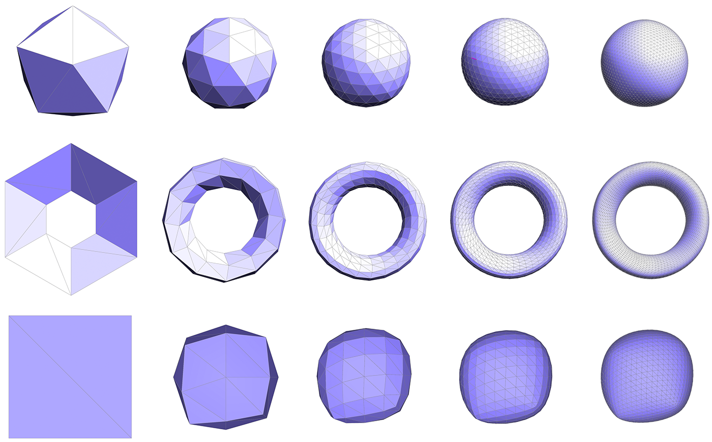
You might try implementing this algorithm in stages, e.g., first see if you can correctly update the connectivity, then worry about getting the vertex positions right. Some examples below illustrate the correct behavior of the algorithm.

---

Simplification

Just as with images, meshes often have far more samples than we really need. The simplification method in Scotty3D simplifies a given triangle mesh by applying quadric error simplification (note that this method is for triangle meshes only!). This method was originally developed at CMU by Michael Garland and Paul Heckbert, in their paper Surface Simplification Using Quadric Error Metrics. (Looking at this paper -- or the many slides and presentations online that reference it -- may be very helpful in understanding and implementing this part of the assignment!)

The basic idea is to iteratively collapse edges until we reach the desired number of triangles. The more edges we collapse, the simpler the mesh becomes. The only question is: which edges should we collapse? And where should we put the new vertex when we collapse an edge? Finding the sequence of edge collapses (and vertex positions) that give an optimal approximation of the surface would be very difficult -- likely impossible! Garland and Heckbert instead proposed a simple, greedy scheme that works quite well in practice, and is the basis of many mesh simplification tools today. Roughly speaking, we're going to write down a function that measures the distance to a given triangle, and then "accumulate" this function as many triangles get merged together.

More precisely, we can write the distance d of a point $x$ to a plane with normal $N$ passing through a point $p$ as

$$d(x) = N \cdot (x - p)$$

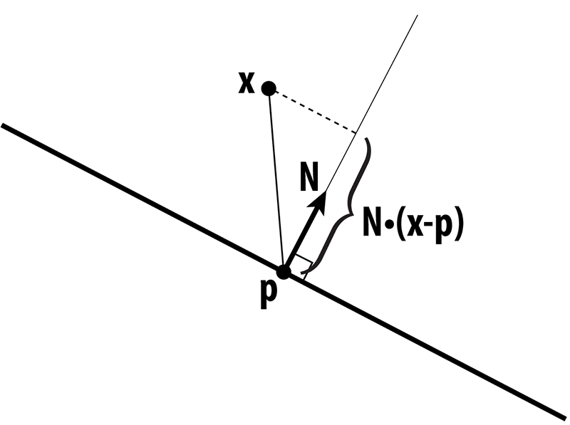
In other words, we measure the extent of the vector from $p$ to $x$ along the normal direction. This quantity gives us a value that is either positive (above the plane), or negative (below the plane). Suppose that $x$ has coordinates $(x,y,z)$, $N$ has coordinates $(a,b,c)$, and let $d = N \cdot p$, then in homogeneous coordinates, the distance to the plane is just

$$u \cdot v$$

where $u = (x,y,z,1)$ and $v = (a,b,c,d)$. When we're measuring the quality of an approximation, we don't care whether we're above or below the surface; just how far away we are from the original surface. Therefore, we're going to consider the square of the distance, which we can write in homogeneous coordinates as

$$(u \cdot v)^2 = u^T v v^T u$$

where $^T$ denotes the transpose of a vector. The term $vv^T$ is an outer product of the vector $v$ with itself, which gives us a symmetric matrix $K = vv^T$. In components, this matrix would look like

a^2   ab    ac   ad
ab    b^2   bc   bd
ac    bc    c^2  cd
ad    bd    cd   d^2

but in Scotty3D it can be constructed by simply calling the method outer( Vector4D, Vector4D ) in matrix4x4.h that takes a pair of vectors in homogeneous coordinates and returns the outer product as a 4x4 matrix. We will refer to this matrix as a "quadric," because it also describes a quadric surface.

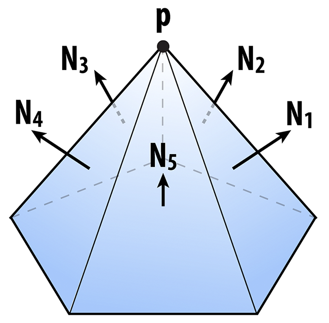
The matrix $K$ tells us something about the distance to a plane. We can also get some idea of how far we are from a vertex by considering the sum of the squared distances to the planes passing through all triangles that touch that vertex. In other words, we will say that the distance to a small neighborhood around the vertex i can be approximated by the sum of the quadrics on the incident faces ijk:

$$K_i = \sum_{\text{all faces ijk touching vertex i}} K_{ijk}$$

Likewise, the distance to an edge ij will be approximated by the sum of the quadrics at its two endpoints:

$$K_{ij} = K_i + K_j$$

In your code, we have added a member Matrix4x4 Face::quadric and Matrix4x4 Vertex::quadric to the faces and vertices of the halfedge mesh. The sums above should then be easy to compute -- you can just add up the Matrix4x4 objects around a vertex or along an edge using the usual "+" operator. You do not need to write an explicit loop over the 16 entries of the matrix.

Once you have a quadric $K$ associated with an edge $ij$, you can ask the following question: if we collapse the edge to a point $x$, where should we put the new point so that it minimizes the (approximate) distance to the original surface? In other words, where should it go so that it minimizes the quantity $x^T K x$?

Just like any other function, we can look for the minimum by taking the derivative with respect to $x$ and setting it equal to zero. (By the way, in this case we're always going to get a minimum and not a maximum because the matrices K are all positive-definite.) In other words, we want to solve the small (4x4) linear system

$$K u = 0$$

for the optimal position $u$, expressed in homogeneous coordinates. We can simplify this situation a bit by remembering that the homogeneous coordinate for a point in 3-space is just 1. After a few simple manipulations, then, we can rewrite this same system as an even smaller 3x3 linear system

$$Ax = b$$

where A is the upper-left 3x3 block of K, and b is minus the upper-right 3x1 column. In other words, the entries of A are just

$$ \left[ \begin{matrix} a^2 & ab & ac \ ab & b^2 & bc \ ac & bc & c^2 \ \end{matrix} \right] $$

and the entries of b are

$$ \left[ \begin{matrix} -ad \ -bd \ -cd \ \end{matrix} \right] $$

The cost associated with this solution can be found by plugging $x$ back into our original expression, i.e., the cost is just

$$x^T K x$$

where $K$ is the quadric associated with the edge. Fortunately, you do not need to write any code to solve this linear system. It can be solved using the method Matrix3x3::inv() which computes the inverse of a 3x3 matrix. In particular, you can write something like this:

Matrix3x3 A; // computed by accumulating quadrics and then extacting the upper-left 3x3 block
Vector3D b;  // computed by extracting minus the upper-right 3x1 column from the same matrix
Vector3D x = A.inv() * b; // solve Ax = b for x, by hitting both sides with the inverse of A

If you're a bit lost at this point, don't worry! There are a lot of details to go through, and we'll summarize everything again in the implementation section. The main idea to keep in mind right now is:

• we're storing a matrix at every vertex that encodes (roughly) the distance to the surface, and
• for each edge, we want to find the point that is (roughly) as close as possible to the surface, according to the matrices at its endpoints.

As we collapse edges, the matrices at endpoints will be combined by just adding them together. So, as we perform more and more edge collapses, these matrices will try to capture the distance to a larger and larger region of the original surface.

The one final thing we want to think about is performance. At each iteration, we want to collapse the edge that results in the least deviation from our original surface. But testing every edge, every single iteration sounds pretty expensive! (Something like O(n^2).) Instead, we're going to put all our edges into a priority queue that efficiently keeps track of the "best" edge for us, even as we add and remove edges from our mesh. In the code framework, we actually introduce a new class called an EdgeRecord that encodes all the essential information about our edge:

// An edge record keeps track of all the information about edges
// that we need while applying our mesh simplification algorithm.
class EdgeRecord {
  public:
    EdgeRecord( void ) {}
    EdgeRecord( EdgeIter& _edge );
    // The second constructor takes an edge, and computes all
    // the essential data.  In particular, it computes the sum
    // of the quadrics at the two endpoints, and solves for the
    // optimal midpoint position as measured by this quadric.
    // It also stores the value of this quadric as the "score"
    // used by the priority queue.

    EdgeIter edge; // the edge referred to by this record

    Vector3D optimalPoint; // the optimal point, if we were
                           // to collapse this edge next

    double cost; // the cost associated with collapsing this edge,
                 // which is very (very!) roughly something like
                 // the distance we'll deviate from the original
                 // surface if this edge is collapsed
};

To initialize an edge record for a given edge, you just have to write

EdgeRecord myRecord(e);

In other words, you hand it the edge to be initialized. This record in turn gets added to a priority queue, which stores all the halfedges, sorted according to the cost of collapsing them:

MutablePriorityQueue queue;
queue.insert(e);

If we ever want to know what the best edge is to collapse, we can just look at the top of the priority queue:

EdgeRecord bestEdge = queue.top();

More documentation is provided in the header file MutablePriorityQueue.h.

Though conceptually sophisticated, quadric error simplification is actually not too hard to implement. It basically boils down to two methods:

EdgeRecord::EdgeRecord( EdgeIter e );            // initializer for an edge record
MeshResampler::downsample( HalfedgeMesh& mesh ); // downsampling via quadric error simplification

As discussed above, the edge record initializer should:

1. Compute a quadric for the edge as the sum of the quadrics at endpoints.
2. Build a 3x3 linear system for the optimal collapsed point, as described above.
3. Solve this system and store the optimal point in EdgeRecord::optimalPoint.
4. Compute the corresponding error value and store it in EdgeRecord::cost.
5. Store the edge in EdgeRecord::edge.

The downsampling routine can then be implemented by following this basic recipe:

1. Compute quadrics for each face by simply writing the plane equation for that face in homogeneous coordinates, and building the corresponding quadric matrix using Matrix4x4::outer(). This matrix should be stored in Face::quadric.
2. Compute an initial quadric for each vertex by adding up the quadrics at all the faces touching that vertex. This matrix should be stored in Vertex::quadric. (Note that these quadrics will get updated as edges are collapsed.)
3. For each edge, create an EdgeRecord and insert it into one global MutablePriorityQueue.
4. Until a target number of triangles is reached, collapse the best/cheapest edge (as determined by the priority queue), and set the quadric at the new vertex to the sum of the quadrics at the endpoints of the original edge. You will also have to update the cost of any edge connected to this vertex.

The algorithm should terminate when a target number of triangles is reached -- for the purpose of this assignment, you should set this number to 1/4th the number of triangles in the input (since subdivision will give you a factor of 4 in the opposite direction). Note that to get the best element from the queue you call MutablePriorityQueue::top(), whereas to remove the best element from the top you must call MutablePriorityQueue::pop() (the separation of these two tasks is fairly standard in STL-like data structures).

As with subdivision, it is critical that you carefully reason about which mesh elements get added/deleted in what order -- particularly in Step 4. A good way to implement Step 4 would be:

1. Get the cheapest edge from the queue.
2. Remove the cheapest edge from the queue by calling pop().
3. Compute the new quadric by summing the quadrics at its two endpoints.
4. Remove any edge touching either of its endpoints from the queue.
5. Collapse the edge.
6. Set the quadric of the new vertex to the quadric computed in Step 2.
7. Insert any edge touching the new vertex into the queue, creating new edge records for each of them.

Note: Step 2 is highlighted, because these instruction used to erroneously recommend that the pop be done at the end. The pop of the cheapest edge needs to occur before any modifications are made to the queue, because otherwise the edge you are processing might not be the cheapest edge at the end of the 7 step process.

Steps 4 and 7 are highlighted because it is easy to get these steps wrong. For instance, if you collapse the edge first, you may no longer be able to access the edges that need to be removed from the queue.

A working implementation should look something like the examples below. You may find it easiest to implement this algorithm in stages. For instance, first get the edge collapses working, using just the edge midpoint rather than the optimal point, then worry about solving for the point that minimizes quadric error.

Isotropic Remeshing

Another thing we might want to do with a mesh is keep the number of samples roughly the same, while improving the shape of individual triangles. The isotropic remeshing algorithm tries to make the mesh as "uniform" as possible, i.e., triangles as close as possible to equilaterial triangles of equal size, and vertex degrees as close as possible to 6 (note: this algorithm is for triangle meshes only). The algorithm you will implement is based on the paper Botsch and Kobbelt, "A Remeshing Approach to Multiresolution Modeling" (Section 4), and can be summarized in just a few simple steps:

1. If an edge is too long, split it.
2. If an edge is too short, collapse it.
3. If flipping an edge improves the degree of neighboring vertices, flip it.
4. Move vertices toward the average of their neighbors.

Repeating this simple process several times typically produces a mesh with fairly uniform triangle areas, angles, and vertex degrees. However, each of the steps deserves slightly more explanation.

Edge Splitting / Collapsing

Ultimately we want all of our triangles to be about the same size, which means we want edges to all have roughly the same length. As suggested in the paper by Botsch and Kobbelt, we will aim to keep our edges no longer than 4/3rds of the mean edge length $L$ in the input mesh, and no shorter than 4/5ths of $L$. In other words, if an edge is longer than 4$L$/3, split it; if it is shorter than 4$L$/5, collapse it. We recommend performing all of the splits first, then doing all of the collapses (though as usual, you should be careful to think about when and how mesh elements are being allocated/deallocated).

Edge Flipping

We want to flip an edge any time it reduces the total deviation from regular degree (degree 6). In particular, let $a_1$, $a_2$ be the degrees of an edge that we're thinking about flipping, and let $b_1$, $b_2$ be the degrees of the two vertices across from this edge. The total deviation in the initial configuration is $|a_1-6| + |a_2-6| + |b_1-6| + |b_2-6|$. You should be able to easily compute the deviation after the edge flip without actually performing the edge flip; if this number decreases, then the edge flip should be performed. We recommend flipping all edges in a single pass, after the edge collapse step.

Vertex Averaging

Finally, we also want to optimize the geometry of the vertices. A very simple heuristic is that a mesh will have reasonably well-shaped elements if each vertex is located at the center of its neighbors. To keep your code clean and simple, we ask that you implement the method Vertex::computeCentroid() which should compute the average position of the neighbors and store it in the member Vertex::centroid. The reason this value must be stored in a temporary variable and not immediately used to replace the current position is similar to the reason we stored temporary vertex positions in our subdivision scheme: we don't want to be taking averages of vertices that have already been averaged. Doing so can yield some bizarre behavior that depends on the order in which vertices are traversed (if you're interested in learning more about this issue, Google around for the terms "Jacobi iterations" and "Gauss-Seidel). So, your code should (i) first compute the centroid for all vertices, and (ii) then update the vertices with new positions.

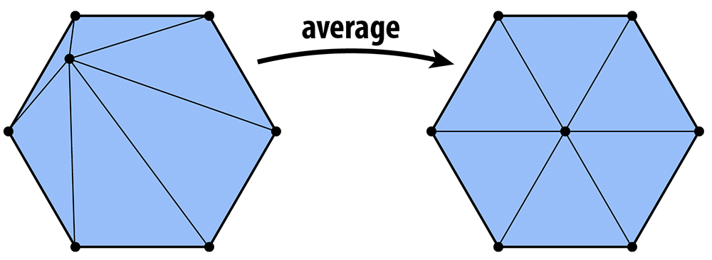
How exactly should the positions be updated? One idea is to simply replace each vertex position with its centroid. We can make the algorithm slightly more stable by moving gently toward the centroid, rather than immediately snapping the vertex to the center. For instance, if p is the original vertex position and c is the centroid, we might compute the new vertex position as $q = p + w(c - p)$ where w is some weighting factor between 0 and 1 (we use 1/5 in the examples below). In other words, we start out at p and move a little bit in the update direction $v = c - p$.

Another important issue here is that if our update direction $v$ has a large normal component, then we'll end up pushing the surface in or out, rather than just sliding our sample points around on the surface. As a result, the shape of the surface will change much more than we'd like (try it!). To ameliorate this issue, we will move the vertex only in the tangent direction, which we can do by projecting out the normal component, i.e., by replacing $v$ with $v - (N \cdot v)N$, where $N$ is the unit normal at the vertex. To get this normal, you will implement the method Vertex::normal(), which computes the vertex normal as the area-weighted average of the incident triangle normals. In other words, at a vertex i the normal points in the direction

$$\sum_{\text{triangles ijk touching vertex i}} A_{ijk} N_{ijk}$$

where $A_{ijk}$ is the area of triangle ijk, and $N_{ijk}$ is its unit normal; this quantity can be computed directly by just taking the cross product of two of the triangle's edge vectors (properly oriented).

Implementation

The final implementation requires very little information beyond the description above; the basic recipe is:

1. Compute the mean edge length $L$ of the input.
2. Split all edges that are longer than 4$L$/3.
3. Collapse all edges that are shorter than 4$L$/5.
4. Flip all edges that decrease the total deviation from degree 6.
5. Compute the centroids for all the vertices.
6. Move each vertex in the tangent direction toward its centroid.

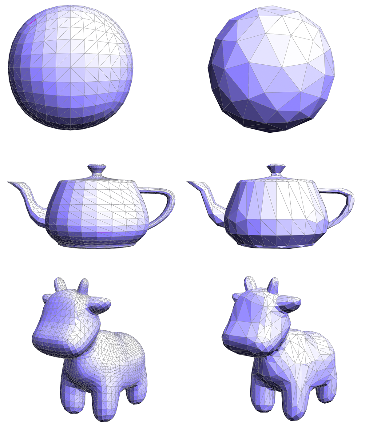
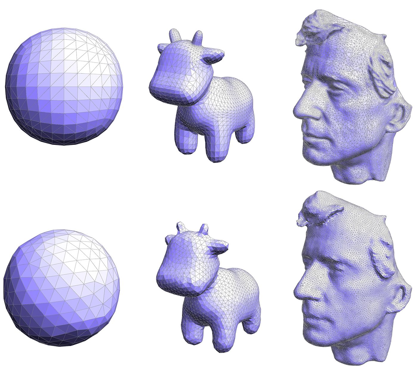
Repeating this procedure about 5 or 6 times should yield results like the ones seen below; you may want to repeat the smoothing step 10-20 times for each "outer" iteration.

Path Tracing

Following the design of modern ray tracing systems, we have chosen to implement the ray tracing components of the Assignment 3 starter code in a very modular fashion. Therefore, unlike previous assignments, your implementation will touch a number of files in the starter code. The main structure of the code base is:

• The main workhorse class is Pathtracer defined in pathtracer.cpp. Inside the ray tracer class everything begins with the method Pathtracer::raytrace_pixel() in pathtracer.cpp. This method computes the value of the specified pixel in the output image.
• The camera is defined in the Camera class in camera.cpp. You will need to modify Camera::generate_ray() in Part 1 of the assignment to generate the camera rays that are sent out into the scene.
• Scene objects (e.g., triangles and spheres) are instances of the Primitive interface defined in static_scene/Primitive.h. You will need to implement the Primitive::intersect() method for both triangles and spheres.
• Lights implement the Light interface defined in static_scene/Light.h. The initial starter code has working implementations of directional lights and constant hemispherical lights.
• Light energy is represented by instances of the Spectrum class. While it's tempting, we encourage you to avoid thinking of spectrums as colors -- think of them as a measurement of energy over many wavelengths. Although our current implementation only represents spectrums by red, green, and blue components (much like the RGB representations of color you've used previously in this class), this abstraction makes it possible to consider other implementations of spectrum in the future. Spectrums can be converted into colors using the Spectrum::toColor() method.
• A major portion of the first half of the assignment concerns implementing a bounding volume hierarchy (BVH) that accelerates ray-scene intersection queries. The implementation of the BVH will be located in bvh.cpp/.h. Note that a BVH is also an instance of the Primitive interface (A BVH is a scene primitive that itself contains other primitives.)

Please refer to the inline comments (or the Doxygen documentation) for further details.

Task 1: Generating Camera Rays

"Camera rays" emanate from the camera and measure the amount of scene radiance that reaches a point on the camera's sensor plane. (Given a point on the virtual sensor plane, there is a corresponding camera ray that is traced into the scene.)

Take a look at Pathtracer::raytrace_pixel() in pathtracer.cpp. The job of this function is to compute the amount of energy arriving at this pixel of the image. Conveniently, we've given you a function Pathtracer::trace_ray(r) that provides a measurement of incoming scene radiance along the direction given by ray r.

When the number of samples per pixel is 1, you should sample incoming radiance at the center of each pixel by constructing a ray r that begins at this sensor location and travels through the camera's pinhole. Once you have computed this ray, then call Pathtracer::trace_ray(r) to get the energy deposited in the pixel.

Step 1: Given the width(frameBuffer.w) and height(frameBuffer.h) of the screen, and point in screen space, compute the corresponding coordinates of the point in normalized ([0-1]x[0x1]) screen space in Pathtracer::raytrace_pixel(). Pass these coordinates to the camera via Camera::generate_ray() in camera.cpp.

Step 2: Implement Camera::generate_ray(). This function should return a ray in world space that reaches the given sensor sample point. We recommend that you compute this ray in camera space (where the camera pinhole is at the origin, the camera is looking down the -Z axis, and +Y is at the top of the screen.) Note that the camera maintains camera-space-to-world space transform c2w that will be handy.

Step 3: Your implementation of Pathtracer::raytrace_pixel() must support supersampling (more than one sample per pixel). The member Pathtracer::ns_aa in the raytracer class gives the number of samples of scene radiance your ray tracer should take per pixel (a.k.a. the number of camera rays per pixel. Note that Pathtracer::gridSampler->get_sample() provides uniformly distributed random 2D points in the [0-1]^2 box (see the implementation in sampler.cpp).

Tips:

• Since it'll be hard to know if you camera rays are correct until you implement primitive intersection, we recommend debugging your camera rays by checking what your implementation of Camera::generate_ray() does with rays at the center of the screen (0.5, 0.5) and at the corners of the image.

• Before starting to write any code, go through the existing code and make sure you understand the camera model we are using.

Extra credit ideas:

• Modify the implementation of the camera to simulate a camera with a finite aperture (rather than a pinhole camera). This will allow your ray tracer to simulate the effect of defocus blur.
• Write your own Sampler2D implementation that generates samples with improved distribution. Some examples include:
  • Jittered Sampling
  • Multi-jittered sampling
  • N-Rooks (Latin Hypercube) sampling
  • Sobol sequence sampling
  • Halton sequence sampling
  • Hammersley sequence sampling

Task 2: Intersecting Triangles and Spheres

Now that your ray tracer generates camera rays, you need to implement ray-primitive intersection routines for the two primitives in the starter code: triangles and spheres. This handout will discuss the requirements of intersecting primitives in terms of triangles.

The Primitive interface contains two types of intersection routines:

• bool Triangle::intersect(const Ray& r) returns true/false depending on whether ray r hits the triangle.

• bool Triangle::intersect(const Ray& r, Intersection *isect) returns true/false depending on whether ray r hits the triangle, but also populates an Intersection structure with information describing the surface at the point of the hit.

You will need to implement both of these routines. Correctly doing so requires you to understand the fields in the Ray structure defined in ray.h.

• Ray.o represents the 3D point of origin of the ray
• Ray.d represents the 3D direction of the ray (this direction will be normalized)
• Ray.min_t and Ray.max_t correspond to the minimum and maximum points on the ray. That is, intersections that lie outside the Ray.min_t and Ray.max_t range should not be considered valid intersections with the primitive.

There are also two additional fields in the Ray structure that can be helpful in accelerating your intersection computations with bounding boxes (see the BBox class in bbox.h). You may or may not find these precomputed values helpful in your computations.

• Ray.inv_d is a vector holding (1/x, 1/d.y, 1/d.z)
• Ray.sin[3] hold indicators of the sign of each component of the ray's direction.

One important detail of the Ray structure is that min_t and max_t are mutable fields of the Ray. This means that these fields can be modified by constant member functions such as Triangle::Intersect(). When finding the first intersection of a ray and the scene, you almost certainly want to update the ray's max_t value after finding hits with scene geometry. By bounding the ray as tightly as possible, your ray tracer will be able to avoid unnecessary tests with scene geometry that is known to not be able to result in a closest hit, resulting in higher performance.

Step 1: Intersecting Triangles

While faster implementations are possible, we recommend you implement ray-triangle intersection using the method described in the lecture slides. Further details of implementing this method efficiently are given in these notes.

There are two important details you should be aware of about intersection:

• When finding the first-hit intersection with a triangle, you need to fill in the Intersection structure with details of the hit. The structure should be initialized with:

  • t: the ray's t-value of the hit point
  • n: the normal of the surface at the hit point. This normal should be the interpolated normal (obtained via interpolation of the per-vertex normals according to the barycentric coordinates of the hit point)
  • primitive: a pointer to the primitive that was hit
  • bsdf: a pointer to the surface brdf at the hit point (obtained via mesh->get_bsdf())

• When intersection occurs with the back-face of a triangle (the side of the triangle opposite the direction of the normal) you should return the normal of triangle pointing away from the side of the triangle that was hit.

• If you need to distinguish back-face-hit and front-face-hit in your implementation, you might consider adding a flag(e.g. bool is_back_hit) to the 'Intersection' structure.

Once you've successfully implemented triangle intersection, you will be able to render many of the scenes in the scenes directory ( /dae)). However, your ray tracer will be very slow!

Step 2: Intersecting Spheres

Please also implement the intersection routines for the Sphere class in sphere.cpp. Remember that your intersection tests should respect the ray's min_t and max_t values.

Task 3: Implementing a Bounding Volume Hierarchy (BVH)

In this task you will implement a bounding volume hierarchy that accelerates ray-scene intersection. All of this work will be in the BVHAccel class in bvh.cpp.

The starter code constructs a valid BVH, but it is a trivial BVH with a single node containing all scene primitives. A BVHNode has the following fields:

• BBox bb: the bounding box of the node (bounds all primitives in the subtree rooted by this node)
• int start: start index of primitives in the BVH's primitive array
• size_t range: range of index in the primitive list (number of primitives in the subtree rooted by the node)
• BVHNode* l: left child node
• BVHNode* r: right child node

The BVHAccel class maintains an array of all primitives in the BVH (primitives). The fields start and range in the BVHNode refer the range of contained primitives in this array.

Step 1: Your job is to construct a BVH using the Surface Area Heuristic discussed in class. Tree construction should occur when the BVHAccel object is constructed.

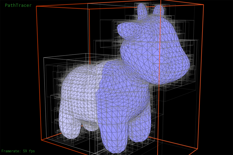
We have implemented a number of tools to help you debug the BVH. Press the V key to enter BVH visualization mode. This mode allows you to directly visualize a BVH as shown below. The current BVH node is highlighted in red. Primitives in the left and right subtrees of the current BVH node are rendered in different colors. Press the LEFT or RIGHT keys to descend to child nodes of the mesh. Press UP to move the parent of the current node.

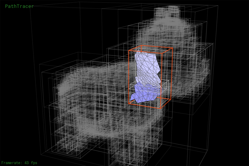
Another view showing the contents of a lower node in the BVH:

Step 2: Implement the ray-BVH intersection routines required by the Primitive interface. You may wish to consider the node visit order optimizations we discussed in class. Once complete, your renderer should be able to render all of the test scenes in a reasonable amount of time.

Task 4: Implementing Shadow Rays

In this task you will modify Pathtracer::trace_ray() to implement accurate shadows.

Currently trace_ray computes the following:

• It computes the intersection of ray r with the scene.
• It computes the amount of light arriving at the hit point hit_p (the irradiance at the hit point) by integrating radiance from all scene light sources.
• It computes the radiance reflected from the hit_p in the direction of -r. (The amount of reflected light is based on the brdf of the surface at the hit point.)

Shadows occur when another scene object blocks light emitted from scene light sources towards the hit point (hit_p). Fortunately, determining whether or not a ray of light from a light source to the hit point is occluded by another object is easy given a working ray tracer (which you have at this point!). You simply want to know whether a ray originating from the hit point (p_hit), and traveling towards the light source (dir_to_light) hits any scene geometry before reaching the light (note, the light's distance from the hit point is given by dist_to_light).

Your job is to implement the logic needed to compute whether hit_p is in shadow with respect to the current light source sample. Below are a few tips:

• A common ray tracing pitfall is for the "shadow ray" shot into the scene to accidentally hit the same triangle as r (the surface is erroneously determined to be occluded because the shadow ray is determined to hit the surface!). We recommend that you make sure the origin of the shadow ray is offset from the surface to avoid these erroneous "self-intersections". For example, o = p_hit + epsilon * dir_to_light (note: EPS_D is defined for this purpose).
• You will find it useful to debug your shadow code using the DirectionalLight since it produces hard shadows that are easy to reason about.

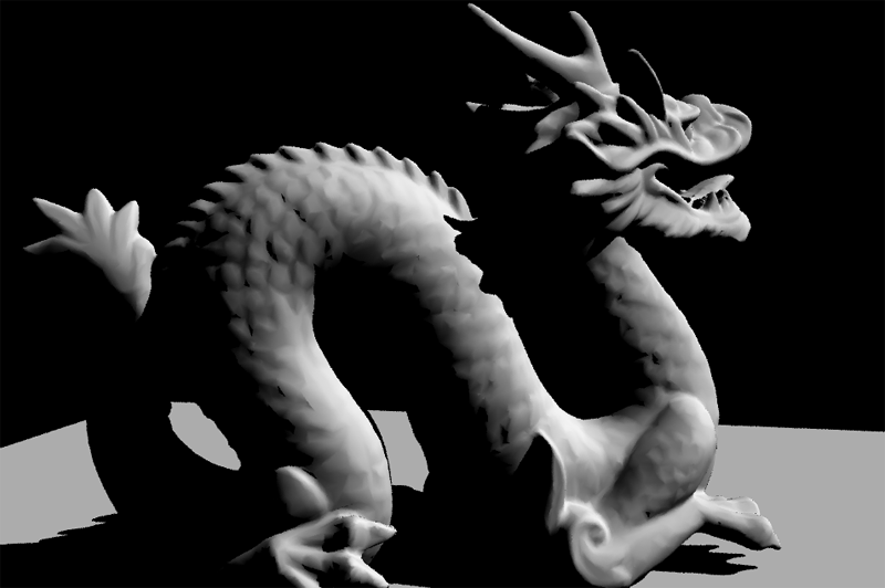
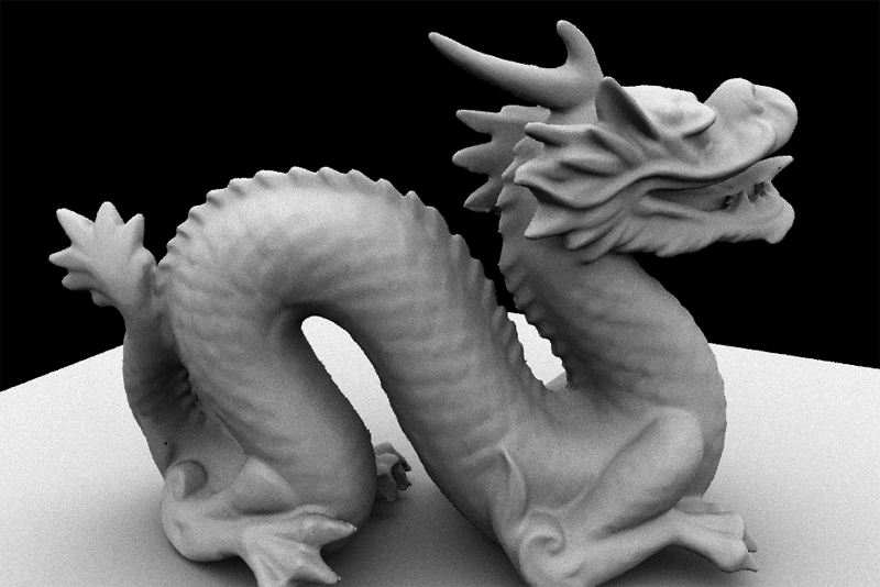
At this point you should be able to render very striking images. For example, here is the Stanford Dragon model rendered with both a directional light and a hemispherical light.

Task 5: Adding Path Tracing

A few notes before getting started:

The new release of the starter code for tasks 5-7 makes a few changes and improvements to the original starter code of the assignment:

• The BRDF class has been renamed BSDF (for "bidirectional scattering distribution function") to indicate that the class is now responsible for computing both light that is reflected from the surface, but also light that is refracted as it is transmitted through the surface. Implementations reside in bsdf.cpp/h.

• Rather than use a single hardcoded light source in your Pathtracer::trace_ray() lights are now defined as part of the scene description file.

You should change your implementation of the reflectance estimate due to direct lighting in Pathtracer::trace_ray() to iterate over the list of scene light sources using the following code:

for (SceneLight* light : scene->lights) { /// do work here... }

• PathTracer::raytrace_pixel(size_t x, size_t y) now returns a Spectrum for the pixel (it doesn't directly update the output image). The update is now handled in PathTracer::raytrace_tile() and is included in the starter code.

---

In this task you will modify your ray tracer to add support for indirect illumination. We wish for you to implement the path tracing algorithm that terminates ray paths using Russian Roulette, as discussed in class. Recommend that you restructure the code in Pathtracer::trace_ray() as follows:

``` Pathtracer::trace_ray() { if (surface hit) { // // compute reflectance due to direct lighting only // for each light: accumulate reflectance contribution due to light

   //
   // add reflectance due to indirect illumination
   //
   randomly select a new ray direction (it may be
   reflection or transmittence ray depending on
   surface type -- see BSDF::sample_f()

   potentially kill path (using Russian roulette)

   evaluate weighted reflectance contribution due
   to light from this direction

} } ```

As a warmup for the next task, implement BSDF::sample_f for diffuse surfaces (DiffuseBSDF:sample_f). The implementation of DiffuseBSDF::f is already provided to you. After correctly implementing diffuse BSDF and path tracing, your renderer should be able to make a beautifully lit picture of the Cornell Box with:

./scotty3d -s 1024 -m 2 -t 8 ../dae/sky/CBspheres_lambertian.dae

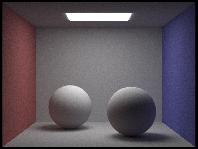
Note the time-quality tradeoff here. With these commandline arguments, your path tracer will be running with 8 worker threads at a sample rate of 256 camera rays per pixel, with a max ray depth of 4. This will produce an image with relatively high quality but will take quite some time to render. Rendering a high quality image will take a very long time as indicated by the image sequence below, so start testing your path tracer early!

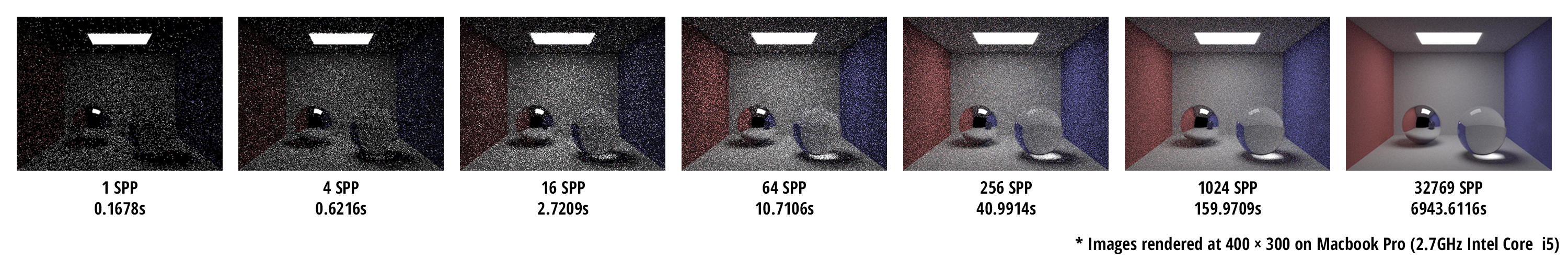
Here are a few tips:

• The termination probability of paths can be determined based on the overall throughput of the path (you'll likely need to add a field to the Ray structure to implement this) or based on the value of the BSDF given wo and wi in the current step. Keep in mind that delta function BRDFs can take on values greater than one, so clamping termination probabilities derived from BRDF values to 1 is wise.

• To convert a Spectrum to a termination probability, we recommend you use the luminance (overall brightness) of the Spectrum, which is available via Spectrum::illum()

• We've given you some pretty good notes on how to do this part of the assignment, but it can still be tricky to get correct.

Task 6: Adding New Materials

Now that you have implemented the ability to sample more complex light paths, it's finally time to add support for more types of materials (other than the fully Lambertian material provided to you in the starter code). In this task you will add support for two types of materials: a perfect mirror and glass (a material featuring both specular reflection and transmittance).

To get started take a look at the BSDF interface in bsdf.cpp. There are a number of key methods you should understand:

• BSDF::f(wo,wi) evaluates the distribution function for a given pair of directions.
• BSDF::sample_f(const Vector3D& wo, Vector3D* wi, float* pdf) generates a random sample wo (which may be a reflection direction or a refracted transmitted light direction). The method returns the value of the distribution function for the pair of directions, and the pdf for the selected sample wi.

There are also two helper functions in the BSDF class that you will need to implement:

• BSDF::reflect(w0, ...) returns a direction wi that is the perfect specular reflection direction corresponding to wi (reflection of w0 about the normal, which in the surface coordinate space is [0,0,1]). More detail about specular reflection is here.

• BSDF::refract(w0, ...) returns the ray that results from refracting the ray w0 about the surface according to Snell's Law. The surface's index of refraction is given by the argument ior. Your implementation should assume that if the ray w0 is entering the surface (that is, if cos(w0,N) > 0) then the ray is currently in vacuum (index of refraction = 1.0). If cos(w0,N) < 0 then your code should assume the ray is leaving the surface and entering vacuum. In the case of total internal reflection, the method should return false.

What you need to do:

1. Implement the class MirrorBSDF which represents a material with perfect specular reflection (a perfect mirror). You should Implement MirrorBSDF::f(), MirrorBSFD::sample_f(), and BSDF::reflect(). (Hint: what should the pdf computed by MirrorBSFD::sample_f() be? What should the reflectance function f() be?)

2. Implement the class GlassBSDF which is a glass-like material that both reflects light and transmit light. As discussed in class the fraction of light that is reflected and transmitted through glass is given by the dielectric Fresnel equations, which are documented in detail here. Specifically your implementation should:

   • Implement BSDF::refract() to add support for refracted ray paths.
   • Use the Fresnel equations to compute the fraction of reflected light and the fraction of transmitted light. Your implementation of
   • Implement GlassBSDF::sample_f(). Your implementation should use the Fresnel equations to compute the fraction of reflected light and the fraction of transmitted light. The returned ray sample should be either a reflection ray or a refracted ray, with the probability of which type of ray to use for the current path proportional to the Fresnel reflectance. (e.g., If the Fresnel reflectance is 0.9, then you should generate a reflection ray 90% of the time. What should the pdf be in this case?)
   • You should read the provided notes on the Fresnel equations as well as on how to compute a transmittance BRDF.

When you are done, you will be able to render images like these:

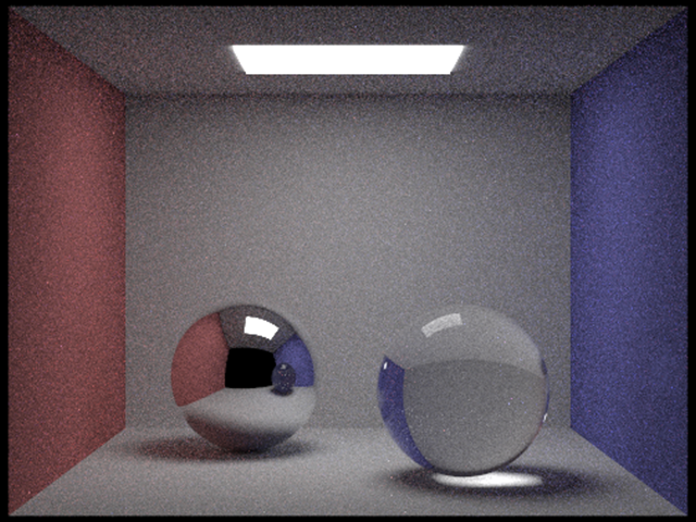
Task 7: Infinite Environment Lighting

The final task of this assignment will be to implement a new type of light source: an infinite environment light. An environment light is a light that supplies incident radiance (really, the light intensity dPhi/dOmega) from all directions on the sphere. The source is thought to be "infinitely far away", and is representative of realistic lighting environments in the real world: as a result, rendering using environment lighting can be quite striking.

The intensity of incoming light from each direction is defined by a texture map parameterized by phi and theta, as shown below.

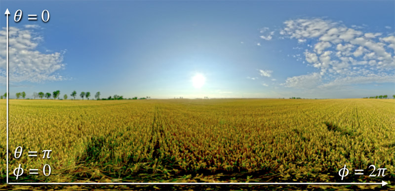
In this task you need to implement the EnvironmentLight::sample_L() method in static_scene/environment_light.cpp. You'll start with uniform direction sampling to get things working, and then move to a more advanced implementation that uses importance sampling to significantly reduce variance in rendered images.

Step one: uniform sampling

To get things working, your first implementation of EnvironmentLight::sample_L() will be quite simple. You should generate a random direction on the sphere (with uniform (1/4pi) probability with respect to solid angle), convert this direction to coordinates (phi, theta) and then look up the appropriate radiance value in the texture map using bilinear interpolation (note: we recommend you begin with bilinear interpolation to keep things simple.)

You an designate rendering to use a particular environment map using the -e commandline parameter: (e.g., -e ../exr/grace.exr )

Since high dynamic range environment maps can be large files, we have not included them in the starter code repo. You can download a set of environment maps from this link.

Tips:

• You must write your own code to uniformly sample the sphere.
• envMap->data contains the pixels of the environment map
• The size of the environment texture is given by envMap->w and envMap->h.

Step two: importance sampling the environment map

Much like light in the real world, most of the energy provided by an environment light source is concentrated in the directions toward bright light sources. Therefore, it makes sense to bias selection of sampled directions towards the directions for which incoming radiance is the greatest. In this final task you will implement an importance sampling scheme for environment lights. For environment lights with large variation in incoming light intensities, good importance sampling will significantly improve the quality of renderings.

The basic idea is that you will assign a probability to each pixel in the environment map based on the total flux passing through the solid angle it represents. We've written up a detailed set of notes for you here (see "Task 7 notes").

Here are a few tips:

• When computing areas corresponding to a pixel, use the value of theta at the pixel centers.
• We recommend precomputing the joint distributions p(phi, theta) and marginal distributions p(theta) in the constructor of EnvironmentLight and storing the resulting values in fields of the class.
• Spectrum::illum() returns the luminance (brightness) of a Spectrum. The probability of a pixel should be proportional to the product of its luminance and the solid angle it subtends.
• std::binary_search is your friend. Documentation is here.