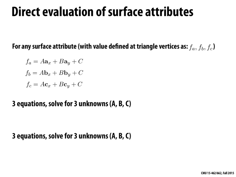
The point if this slide is that for a triangle with vertices in 2D, you can compute the value of any attribute as an affine function of screen space (x,y). I alluded to this in the bottom right of [slide 19](http://15462.courses.cs.cmu.edu/fall2015/lecture/texture/slide_019 just by rearranging terms of the barycentric interpolation equation). However, be careful. On the next slide I point that that this only holds true for triangles with vertices in the same Z-plane. For triangles that are not edge on with the camera, it's not $f$ that's affine in (x,y), its the ratio f/w. So f_a, f_b, f_c above are really f_a/w, f_b/w, f_c/w.
While your first reaction to this approach might be "Ick, solving a 3x3 linear system per attribute sounds expensive, I'd rather compute barycentric coordinates once using one of the previous methods and then use those coefficients to interpolate all attributes."
However, the following is a very efficient way to compute the "2D plane equations" for each surface attribute of the triangle. (Note that interpolating a quantity like a color involves 3 attribute equations, one each for R, G, and B.).
Now rewrite the equations in a coordinate system with $\begin{bmatrix}\mathbf{a}_x & \mathbf{a}_y \end{bmatrix}$ at the origin. (Note this is a good thing to do for numerical stability anyways, as in floating point math you have greater precision near the origin.) The result is:
Carrying the math all the way through, we have:
$$
\begin{bmatrix}
A \\
B
\end{bmatrix} =
\frac{1}{(\mathbf{b}_x-\mathbf{a}_x)(\mathbf{c}_y-\mathbf{a}_y) - (\mathbf{c}_x-\mathbf{a}_x)(\mathbf{b}_y-\mathbf{a}_y)}
\begin{bmatrix}
\mathbf{c}_y-\mathbf{a}_y & \mathbf{a}_y-\mathbf{b}_y \\
\mathbf{a}_x-\mathbf{c}_x & \mathbf{b}_x-\mathbf{a}_x
\end{bmatrix}
\begin{bmatrix}
f_2-f_1 \\
f_3-f_1 \\
\end{bmatrix}
$$
$$
= \mathbf{M}\begin{bmatrix}
f_2-f_1 \\
f_3-f_1 \\
\end{bmatrix}
$$
Note that the matrix $\mathbf{M}$ is dependent only on the edges of the triangle and not on the values of individual surface attributes. In fact, its entries are just the edge slopes and must be computed anyway as part of generating the edge equations needed for coverage sampling. Therefore, $\mathbf{M}$ is computed once per triangle and reused for computing the 2D plane equations for all attributes. Modern OpenGL and Direct3D GPU pipelines support up to 32 float4 values as attributes, equivalent to 128 scalar attributes per triangle.
This minimal setup, plus the efficiency of evaluating the attribute equations on a per sample basis, as described on slide 25, make rasterization very efficient.
The point if this slide is that for a triangle with vertices in 2D, you can compute the value of any attribute as an affine function of screen space (x,y). I alluded to this in the bottom right of [slide 19](http://15462.courses.cs.cmu.edu/fall2015/lecture/texture/slide_019 just by rearranging terms of the barycentric interpolation equation). However, be careful. On the next slide I point that that this only holds true for triangles with vertices in the same Z-plane. For triangles that are not edge on with the camera, it's not $f$ that's affine in (x,y), its the ratio f/w. So f_a, f_b, f_c above are really f_a/w, f_b/w, f_c/w.
While your first reaction to this approach might be "Ick, solving a 3x3 linear system per attribute sounds expensive, I'd rather compute barycentric coordinates once using one of the previous methods and then use those coefficients to interpolate all attributes."
However, the following is a very efficient way to compute the "2D plane equations" for each surface attribute of the triangle. (Note that interpolating a quantity like a color involves 3 attribute equations, one each for R, G, and B.).
In matrix form the linear system looks like:
$$ \begin{bmatrix} \mathbf{a}_x & \mathbf{a}_y & 1 \\ \mathbf{b}_x & \mathbf{b}_y & 1 \\ \mathbf{c}_x & \mathbf{c}_y & 1 \end{bmatrix} \begin{bmatrix} A \\ B \\ C \end{bmatrix} = \begin{bmatrix} f_1 \\ f_2 \\ f_3 \end{bmatrix} $$
Now rewrite the equations in a coordinate system with $\begin{bmatrix}\mathbf{a}_x & \mathbf{a}_y \end{bmatrix}$ at the origin. (Note this is a good thing to do for numerical stability anyways, as in floating point math you have greater precision near the origin.) The result is:
$$ \begin{bmatrix} 0 & 0 & 1 \\ \mathbf{b}_x-\mathbf{a}_x & \mathbf{b}_y-\mathbf{a}_y & 1 \\ \mathbf{c}_x-\mathbf{a}_x & \mathbf{c}_y-\mathbf{a}_y & 1 \end{bmatrix} \begin{bmatrix} A \\ B \\ C \end{bmatrix} = \begin{bmatrix} f_1 \\ f_2 \\ f_3 \end{bmatrix} $$
This implies $C = f_1$ and A and B can be obtained by solving the simpler 2x2 system:
$$ \begin{bmatrix} \mathbf{b}_x-\mathbf{a}_x & \mathbf{b}_y-\mathbf{a}_y \\ \mathbf{c}_x-\mathbf{a}_x & \mathbf{c}_y-\mathbf{a}_y \end{bmatrix} \begin{bmatrix} A \\ B \\ \end{bmatrix} = \begin{bmatrix} f_2 - f_1 \\ f_3 - f_1 \end{bmatrix} $$
Carrying the math all the way through, we have: $$ \begin{bmatrix} A \\ B \end{bmatrix} = \frac{1}{(\mathbf{b}_x-\mathbf{a}_x)(\mathbf{c}_y-\mathbf{a}_y) - (\mathbf{c}_x-\mathbf{a}_x)(\mathbf{b}_y-\mathbf{a}_y)} \begin{bmatrix} \mathbf{c}_y-\mathbf{a}_y & \mathbf{a}_y-\mathbf{b}_y \\ \mathbf{a}_x-\mathbf{c}_x & \mathbf{b}_x-\mathbf{a}_x \end{bmatrix} \begin{bmatrix} f_2-f_1 \\ f_3-f_1 \\ \end{bmatrix} $$ $$ = \mathbf{M}\begin{bmatrix} f_2-f_1 \\ f_3-f_1 \\ \end{bmatrix} $$
Note that the matrix $\mathbf{M}$ is dependent only on the edges of the triangle and not on the values of individual surface attributes. In fact, its entries are just the edge slopes and must be computed anyway as part of generating the edge equations needed for coverage sampling. Therefore, $\mathbf{M}$ is computed once per triangle and reused for computing the 2D plane equations for all attributes. Modern OpenGL and Direct3D GPU pipelines support up to 32 float4 values as attributes, equivalent to 128 scalar attributes per triangle.
This minimal setup, plus the efficiency of evaluating the attribute equations on a per sample basis, as described on slide 25, make rasterization very efficient.