Question 1
Describe why sampling a signal more densely is one way to reduce aliasing. Is there a downside of increasing the rate at which a signal is sampled?
Solution:
Consider an input signal has high-frequency information that is not observed by a set of coarse measurements. In other words, features of the signal "fall between" the measurements, such as the sharp rise in the function that occurs between the measurements at x2 and x3 in slide 11. Since these high-frequency details are not represented in the measurements, reconstruction of the sampled signal yields a low-frequency signal, such as that shown on slide 14 or in the bottom example on slide 44 where a reconstruction of a sampled high frequency sine curve is shown. Aliasing is a phenomenon where high-frequency components of an input signal falsely appear as low-frequency details after reconstruction. (Hence the name "aliasing"!) In addition to slide 44, an excellent example of aliasing is shown on slide 49. Sampling the signal more densely allows for measurement of finer and finer scale details in the input signal. Correspondingly, the resulting reconstruction is more accurate.
Of course, there's a computational cost to increasing sampling density: more samples must be stored in a computer, increasing the amount of required storage and the cost of processing and communication of this information. (High-resolution photos look great on Facebook but can be a pain to upload on a bad data connection!)
For those curious, we've primarily been using aliasing to describe artifacts due to undersampling in this lecture. In reality, there are two causes for aliasing: (1) undersampling and (2) imperfect reconstruction (using reconstruction filters other than a sinc). Aliasing due to undersampling is called prealiasing and errors in reconstruction due to approximation of an idela filter are called post-aliasing. In general, aliasing is used to refer to artifacts due to either source of errors.
Question 2
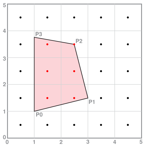
Consider a quadrilateral with the following vertex positions. (You should assume the vertices are connected in the order they are listed.)
P0=(1  , 1   )
P1=(3  , 1.5 )
P2=(2.5, 3.5 )
P3=(1  , 3.75)
- Derive the implicit edge equation for the edge between P0 and P1.
- Assuming coverage sample points are uniformally distributed in the domain at half-integer coordinates (0.5, 0.5), (1.5, 0.5), etc., how many sample points are covered by the given quadrilateral? For simplicity, assume that a sample point on an edge is considered to be within the quadrilateral.
Solution:
The edge equation $E(x,y) = Ax + By = C$ for the line connecting P0=(1,1) and P1=(3, 1.5) can be derived by plugging P0 and P1 into the point-slope equation of a line.
$E(x,y) = (x - 1)(1.5 - 1) - (y - 1)(3 - 1)$
$E(x,y) = 0.5x - 2y + 1.5$
The figure below illustrates the specified quadrilateral on a coordinate grid. Positions of screen coverage sample points are given by the dots. (Notice they are at half-integer coordinates as specified in the problem.) Sample points inside the shape are highlighted in red. There are six covered points. Note that the sample point at (2.5, 3.5) coincides with vertex P2 of the quadrilateral and thus lies on two edges. Since the question specifies that any sample point falling on an edge should be considered to be covered by the shape, this point is covered.