Overview

This document describes the internal data structures and algorithms that comprise the Scotty3D codebase, focusing mainly on core functionality (e.g., meshing and ray tracing). Limited documentation of the graphical user interface (GUI) is available via comments in the source itself (though this information is not needed for assignments).

Animator

Task 1 - Spline Interpolation

As we discussed in class, data points in time can be interpolated by constructing an approximating piecewise polynomial or spline. In this assignment you will implement a particular kind of spline, called a Catmull-Rom spline. A Catmull-Rom spline is a piecewise cubic spline defined purely in terms of the points it interpolates. It is a popular choice in real animation systems, because the animator does not need to define additional data like tangents, etc. (However, your code may still need to numerically evaluate these tangents after the fact; more on this point later.) All of the methods relevant to spline interpolation can be found in spline.h with implementations in spline.inl.

Task 1a - Hermite Curve over the Unit Interval

Recall that a cubic polynomial is a function of the form

$$p(t) = at^3 + bt^2 + ct + d$$

where $a, b, c$, and $d$ are fixed coefficients. However, there are many different ways of specifying a cubic polynomial. In particular, rather than specifying the coefficients directly, we can specify the endpoints and tangents we wish to interpolate. This construction is called the "Hermite form" of the polynomial. In particular, the Hermite form is given by

$$p(t) = h_{00}(t)p_0 + h_{10}(t)m_0 + h_{01}(t)p_1 + h_{11}(t)m_1$$

where $p_0,p_1$ are the endpoint positions, $m_0,m_1$ are the endpoint tangents, and $h_{ij}$ are the Hermite bases

$$h_{00}(t) = 2t^3 - 3t^2 + 1$$

$$h_{10}(t) = t^3 - 2t^2 + t$$

$$h_{01}(t) = -2t^3 + 3t^2$$

$$h_{11}(t) = t^3 - t^2$$

Your first task is to implement the method Spline::cubicSplineUnitInterval(), which evaluates a spline defined over the time interval $[0,1]$ given a pair of endpoints and tangents at endpoints. Optionally, the user can also specify that they want one of the time derivatives of the spline (1st or 2nd derivative), which will be needed for our dynamics calculations.

Your basic strategy for implementing this routine should be:

• Evaluate the time, its square, and its cube. (For readability, you may want to make a local copy
• Using these values, as well as the position and tangent values, compute the four basis functions $h_{00}, h_{01}, h_{10},$ and $h_{11}$ of a cubic polynomial in Hermite form. Or, if the user has requested the nth derivative, evaluate the nth derivative of each of the bases.
• Finally, combine the endpoint and tangent data using the evaluated bases, and return the result.

Notice that this function is templated on a type T. In C++, a templated class can operate on data of a variable type. In the case of a spline, for instance, we want to be able to interpolate all sorts of data: angles, vectors, colors, etc. So it wouldn't make sense to rewrite our spline class once for each of these types; instead, we use templates. In terms of implementation, your code will look no different than if you were operating on a basic type (e.g., doubles). However, the compiler will complain if you try to interpolate a type for which interpolation doesn't make sense! For instance, if you tried to interpolate Skeleton objects, the compiler would likely complain that there is no definition for the sum of two skeletons (via a + operator). In general, our spline interpolation will only make sense for data that comes from a vector space, since we need to add T values and take scalar multiples.

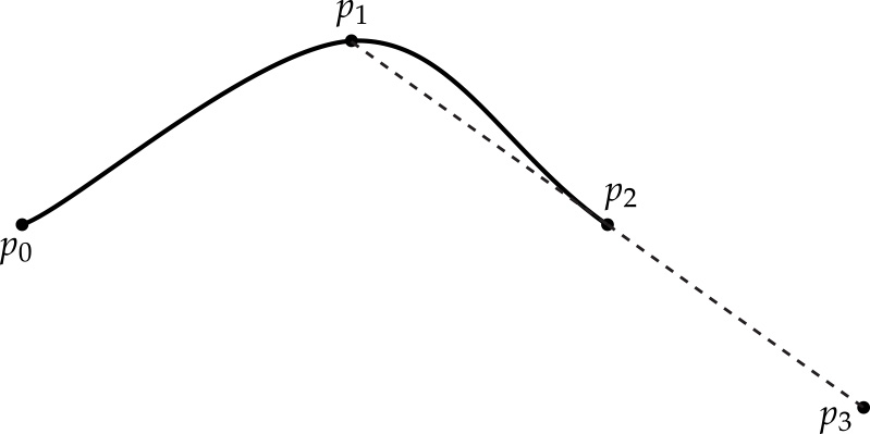
Task 1B: Evaluation of a Catmull-Rom spline

Using the routine from part 1A, you will now implement the method Spline::evaluate() which evaluates a general Catmull-Rom spline (and possibly one of its derivatives) at the specified time. Since we now know how to interpolate a pair of endpoints and tangents, the only task remaining is to find the interval closest to the query time, and evaluate its endpoints and tangents.

The basic idea behind Catmull-Rom is that for a given time t, we first find the four closest knots at times

$$t_0 < t_1 \leq t < t_2 < t_3$$

We then use t1 and t2 as the endpoints of our cubic "piece," and for tangents we use the values

$$m_1 = ( p_2 - p_0 ) / (t_2 - t_0)$$

$$m_2 = ( p_3 - p_1 ) / (t_3 - t_1)$$

In other words, a reasonable guess for the tangent is given by the difference between neighboring points. (See the Wikipedia and our course slides for more details.)

This scheme works great if we have two well-defined knots on either side of the query time t. But what happens if we get a query time near the beginning or end of the spline? Or what if the spline contains fewer than four knots? We still have to somehow come up with a reasonable definition for the positions and tangents of the curve at these times. For this assignment, your Catmull-Rom spline interpolation should satisfy the following properties:

• If there are no knots at all in the spline, interpolation should return the default value for the interpolated type. This value can be computed by simply calling the constructor for the type: T(). For instance, if the spline is interpolating Vector3D objects, then the default value will be $(0,0,0)$.
• If there is only one knot in the spline, interpolation should always return the value of that knot (independent of the time). In other words, we simply have a constant interpolant. (What, therefore, should we return for the 1st and 2nd derivatives?)
• If the query time is less than or equal to the initial knot, return the initial knot's value. (What do derivatives look like in this region?)
• If the query time is greater than or equal to the final knot, return the final knot's value. (What do derivatives look like in this region?)

Once we have two or more knots, interpolation can be handled using general-purpose code. In particular, we can adopt the following "mirroring" strategy to obtain the four knots used in our computation:

• Any query time between the first and last knot will have at least one knot "to the left" $(k_1)$ and one "to the right" $(k_2)$.
• Suppose we don't have a knot "two to the left" $(k_0)$. Then we will define a "virtual" knot $k_0 = k_1 - (k_2-k_1)$. In other words, we will "mirror" the difference be observe between $k_1$ and $k_2$ to the other side of $k_1$.
• Likewise, if we don't have a knot "two to the left" of $t (k_3)$, then we will "mirror" the difference to get a "virtual" knot $k_3 = k_2 + (k_2-k_1)$.
• At this point, we have four valid knot values (whether "real" or "virtual"), and can compute our tangents and positions as usual.
• These values are then handed off to our subroutine that computes cubic interpolation over the unit interval.

An important thing to keep in mind is that Spline::cubicSplineUnitInterval() assumes that the time value t is between 0 and 1, whereas the distance between two knots on our Catmull-Rom spline can be arbitrary. Therefore, when calling this subroutine you will have to normalize t such that it is between 0 and 1, i.e., you will have to divide by the length of the current interval over which you are interpolating. You should think very carefully about how this normalization affects the value and derivatives computed by the subroutine, in comparison to the values and derivatives we want to return.

Internally, a Spline object stores its data in an STL map that maps knot times to knot values. A nice thing about an STL map is that it automatically keeps knots in sorted order. Therefore, we can quickly access the knot closest to a given time using the method map::upper_bound(), which returns an iterator to knot with the smallest time greater than the given query time (you can find out more about this method via online documentation for the Standard Template Library).

Using the splines

Once you have splines implemented, you should be able to move entire objects around the scene at different points on the timeline, and all aspects of it should be smoothly interpolated (e.g. position, rotation and scale).

Task 2 - Skeleton Kinematics

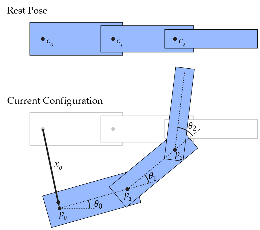
A Skeleton is what we use to drive our animation. You can think of them like the set of bones we have in our own bodies and joints that connect these bones. For convenience, we have merged the bones and joints into the Joint class which holds the orientation of the joint relative to its parent in its rotation, and axis representing the direction and length of the bone with respect to its parent Joint. Each Mesh has an associated Skeleton class which holds a rooted tree of Joints, where each Joint can have an arbitrary number of children.

All of our joints are ball Joints which have a set of 3 rotations around the $x$, $y$, and $z$ axes, called Euler angles. Whenever you deal with angles in this way, a fixed order of operations must be enforced, otherwise the same set of angles will not represent the same rotation. In order to get the full rotational transformation matrix, $R$, we can create individual rotation matrices around the $X$, $Y$, and $Z$ axes, which we call $R_x$, $R_y$, and $R_z$ respectively. The particular order of operations that we adopted for this assignment is that $R := R_x * R_y * R_z$.

Task 2a - Forward Kinematics

When a joint's parent is rotated, that transformation should be propagated down to all of its children. In the diagram below, $c_0$ is the parent of $c_1$ and $c_1$ is the parent of $c_2$. When a translation of $x_0$ and rotation of $\theta_0$ is applied to $c_0$, all of the descendants are affected by this transformation as well. Then, $c_1$ is rotated by $\theta_1$ which affects itself and $c_2$. Finally, when rotation of $\theta_2$ is applied to $c_2$, it only affects itself because it has no children.

You need to implement these routines in dynamic_scene/joint.cpp for forward kinematics.

• Joint::getTransformation()
  Returns the transformation up to the base of this joint (end of its parent joint). Joint is a child class of SceneObject which has its own version of getTransformation() that you can use by calling SceneObject::getTransformation(). As explained above, a joint's transformation is accumulated as you traverse the hierarchy of joints. You should traverse upwards from this joint's parent all the way up to the root joint and accumulate their transformations. Also, make sure to apply the mesh's transformation at the end, accessible with skeleton->mesh->getTransformation().
• Joint::getBasePosInWorld()
  Returns the base position of the joint in world coordinate frame.
• Joint::getEndPosInWorld()
  Returns the end position of the joint in world coordinate frame.

Task 2b - Inverse Kinematics

Single Target IK

Now that we have a logical way to move joints around, we can implement Inverse Kinematics, which will move the joints around in order to reach a target point. There are a few different ways we can do this, but for this assignment we'll implement an iterative method called gradient descent in order to find the minimum of a function. For a function $f: \mathbb{R}^n \to \mathbb{R}$, we'll have the update scheme:

$$X_{k+1} = X_k - \tau \nabla f$$

Where $\tau$ is a small timestep. For this task, we'll be using gradient descent to find the minimum of the cost function:

$$f(\theta(t)) = \frac{1}{2}|p(\theta(t)) - q|^2$$

Where $p(\theta(t))$ is the position in world space of the target joint, and $q$ is the position in world space of the target point.

More specifically, we'll be using a technique called Jacobian Transpose, which relies on the assumption that:

$$\nabla_\theta f \approx \alpha J_\theta^T (p(\theta) - q)$$

Where:

• $\theta$ (n x 1) is the function $\theta(t) = (\theta_1(t),\ldots,\theta_n(t))$, where $\theta_i(t)$ is the angle of joint $i$ around the axis of rotation
• $\alpha$ is a constant
• $J_\theta$ (3 x n) is the Jacobian of $\theta$

Note that here $n$ refers to the number of joints in the skeleton. Although in reality this can be reduced to just the number of joints between the target joint and the root, inclusive, because all joints not on that path should stay where they are, so their columns in $J_\theta$ will be 0. So $n$ can just be the number of joints between the target and the root, inclusive. Additionally note that since this will get multiplied by $\tau$ anyways, you can ignore the value of $\alpha$, and just consider the timestep as $\tau_2 = \tau * \alpha$.

Now we just need a way to calcluate the Jacobian of $\theta$. For this, we can use the fact that:

$$(J_\theta)_i = \vec{r} \times \vec{p}$$

Where:

• $J_i$ is the $i^{th}$ column of $(J_\theta)$
• $\vec{r}$ is the axis of rotation
• $\vec{p}$ is the vector from the base of joint $i$ to the end point of the target joint

For a more in-depth derivation of Jacobian transpose (and a look into other inverse kinematics algorithms), please check out this presentation. (Pages 61-69 in particular)

Now, all of this will work for updating the angle along a single axis, but we have 3 axes to deal with. Luckily, extending it to 3 dimensions isn't very difficult, we just need to update the angle along each axis independently.

Multi-Target

We'll extend this so we can have multiple targets, which will then use the function to minimize:

$$f(\theta(t)) = \frac{1}{2}\sum_i |p_i(\theta(t)) - q_i|^2$$

which is a simple extension actually. Since each term is independent and added together, we can get the gradient of this new cost function just by summing the gradients of each of the constituent cost functions!

You should implement multi-target IK, which will take a std::map of Joints and target points for that joint. Each joint can only have 1 target point.

In order to implement this, you should update Joint::calculateAngleGradient and Skeleton::reachForTarget. Joint::calculateAngleGradient should calculate the gradient of $\theta$ in the x,y, and z directions, and add them to Joint::ikAngleGradient for all relevant joints. Skeleton::reachForTarget should actually do the gradient descent calculations and update the angles of each joint, saving them with Joint::setAngle. In this function, you should probably use a very small timestep, but do several iterations of gradient descent in order to speed things up. For even faster and better results, you can also implement a variable timestep instead of just using a fixed one. Note also that the root joint should never be updated.

A key thing for this part is to remember what coordinate frame you're in, because if you calculate the gradients in the wrong coordinate frame or use the axis of rotation in the wrong coordinate frame your answers will come out very wrong!

Task 3 - Linear Blend Skinning

Now that we have a skeleton set up, we need to link the skeleton to the mesh in order to get the mesh to follow the movements of the skeleton. We will implement linear blend skinning in Mesh::linearBlendSkinning().

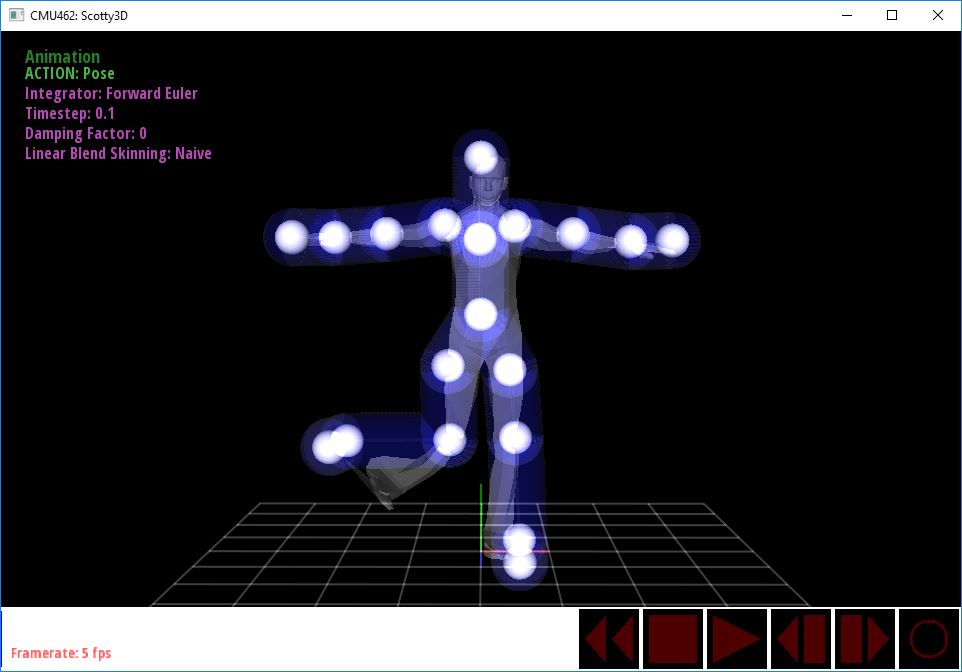
Task 3a Naive Linear Blend Skinning

The easiest way to do this is to update each of mesh vertices' positions in relation to the bones (Joints) in the skeleton. You should compute each vertex's position with respect to each joint j in the skeleton in j's coordinate frame when no transformations have been applied to the skeleton (bind pose). Then, you should find where this vertex would end up with respect to joint j after all of the joints in the skeletons have been transformed if it were to have the same relative position in j's coordinate frame. Also, for this vertex, you should find the closest point on joint j's bone segment (axis) and store the distance to the closest point. Structure called LBSInfo has been defined for you in dynamic_scene/mesh.h to store these information. Now, you can compute the final position of the vertex by doing a weighted average with respect to the inverse distance (closer bones should have more influence on the position of the vertex).

Below we have an equation representation. $v_i$ is the new vertex position. $w_{ij}$ is the weight metric computed as the inverse of distance between vertex $i$ and closest point on joint $j$. $v_i^j$ is the vertex's position with respect to joint $j$ after joint's transformations has been applied.

$$v_{i} = \sum_{j}{w_{ij}v_i^j}$$

$$w_{ij} = \frac{\frac{1}{dist_{ij}}}{\sum_{j}{\frac{1}{dist_{ij}}}}$$

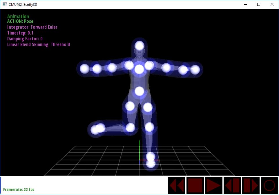
Task 3b Linear Blend Skinning with Threshold

After you implemented the method in Task 3a, you probably noticed that parts of the mesh that is very far away moves when you move a joint. In part 3b, we will implement a threshold to limit the volume that each joint affects. You should change your code such that when parameter useCapsuleRadius is true, you check the distance between the vertex and the closest point on the joint, and if it is more than the joint's capsuleRadius, you do not let that joint affect this vertex.

Naive linear blend skinning affects other parts of the mesh, not just the leg. Also, the leg does not follow the joint exactly because other joints hold it back.

Linear blend skinning with threshold allows us to better pose our characters.

Task 4 - Physical Simulation

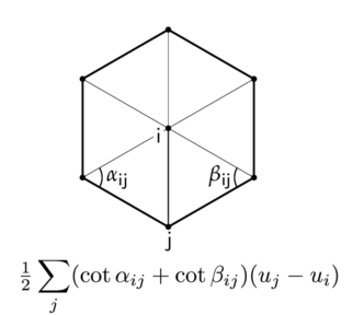
The next task is to implement an integrator for the (undamped) wave equation across a mesh: $$u'' = \Delta u$$

We've discussed in class how to calculate the Discrete Laplacian operator, via the cotan-formula: $$\Delta u = \frac{1}{2}\sum_j (\cot \alpha_{ij} + \cot \beta_{ij})(u_j - u_i)$$

For this task, you should update Vertex::Laplacian in halfedgeMesh.cpp and Mesh::forwardEuler and Mesh::symplecticEuler in dynamic_scene/mesh.cpp, storing your calculated u value in Vertex::offset and the calculated u' value in Vertex::velocity. Be careful about when you update these quantities. Note that since forward Euler is defined to solve a single, first-order differential equation, solving a second-order one will require you to break it up into 2 first order equations and solve each of them with forward Euler.

The next task is to change your intergrators to solve the damped wave equation across a mesh: $$u'' = \Delta u - \lambda u'$$ Where we call $\lambda$ the damping factor, which can take on any value between 0 and 1. You'll notice here that a damping factor of 0 is identical to the undamped case.

Once you've implemented these integrators, you can switch between them with F and S, change the timestep with - and =, and the damping factor with SHIFT/- and SHIFT/=. Be aware that Forward Euler is not numerically stable, so if your solutions blow up then it's the expected behavior.

Task 5 - Get Creative!

Now that you have an awesome animation system, make an awesome animation! You have 2 options on how to render your animation, you can use t (or T) to save the video with rasterization, or n (or N) to save the video with your raytracer, either one is fine! Once you've rendered all the frames of your video, you can combine them into a video by using:

ffmpeg -r 60 -f image2 -s 800x600 -i ./Video_[TIME]_%4d.png -vcodec libx264 out.mp4

Where [TIME] should be replaced by the timestamp in each frame's filename (they should all be identical). If you don't have ffmpeg installed on your system, you can get it through most package managers, or you can download it directly, or use your own video creation program.

Have fun!